The article below was contributed by Timothy Malche, an assistant professor in the Department of Computer Applications at Manipal University Jaipur.

SIFT (Scale-Invariant Feature Transform) is a computer vision algorithm designed to detect and describe local features in images. Developed by David Lowe, it has become one of the most widely used algorithms for feature detection, object recognition, and image matching due to its robustness in handling scaling, rotation, and minor changes in illumination or viewpoint.

The core objective of SIFT is to detect distinctive and invariant keypoints in images and generate robust descriptors that can be used to match those keypoints across different images. The algorithm achieves scale invariance, meaning it can detect the same features regardless of the image’s scale. Additionally, it is rotation invariant, which means the keypoints detected remain consistent even if the image is rotated.

How The SIFT Algorithm Works

The SIFT algorithm is designed to detect distinctive features, called keypoints, in images. These keypoints are unique areas that can be used to recognize objects in different images, even if the image is scaled, rotated, or slightly changed. Following are the main steps in the SIFT algorithm:

• Scale-space Extrema Detection
• Keypoint Localization
• Orientation Assignment
• Keypoint Descriptor

Here’s a step-by-step explanation of how the SIFT algorithm works:

Step #1: Scale-Space Extrema Detection

In this step keypoints (features) across different scales of the image are detected. The scale space is the process of creating a set of progressively blurred images at multiple resolutions to detect keypoints that are scale-invariant (they remain the same even if the image size changes). It helps to detect features that are stable and can be recognized even when the image is scaled or resized. Let's understand how it works. 

First, algorithm progressively applies a gaussian blur to the image to blur it at different scales (levels), which smooths it by different amounts. This means we see the image from clear to blurry. This can be described mathematically as:

L(x,y,σ)=G(x,y,σ)∗I(x,y)

Where:

• L(x,y,σ) is the blurred image at scale σ.
• G(x,y,σ) is the Gaussian kernel.
• I(x,y) is the original image.

The image is also downsampled (reduced in size) after each octave, allowing features to be detected at smaller resolutions (or sizes) as well. Here, octave is a set of images at different resolutions.

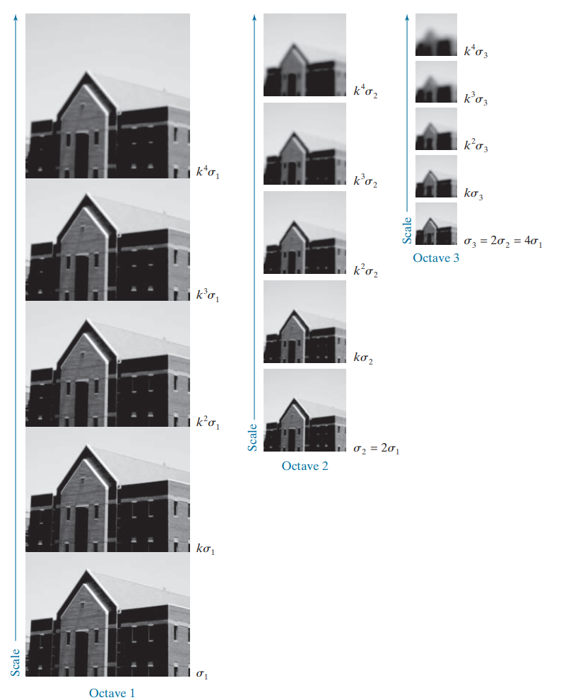
The image below shows how an image is progressively blurred across different scales and octaves. Each octave represents a set of images at progressively lower resolutions (downsampled). Within each octave, the image is blurred by different amounts.  The leftmost column shows the images in Octave 1, starting with the original image at the bottom and becoming more blurred as you move upward. The middle column represents Octave 2, where the image has been downsampled (reduced in size) and similarly blurred at different scales. The rightmost column shows Octave 3, where the image is further downsampled and blurred.

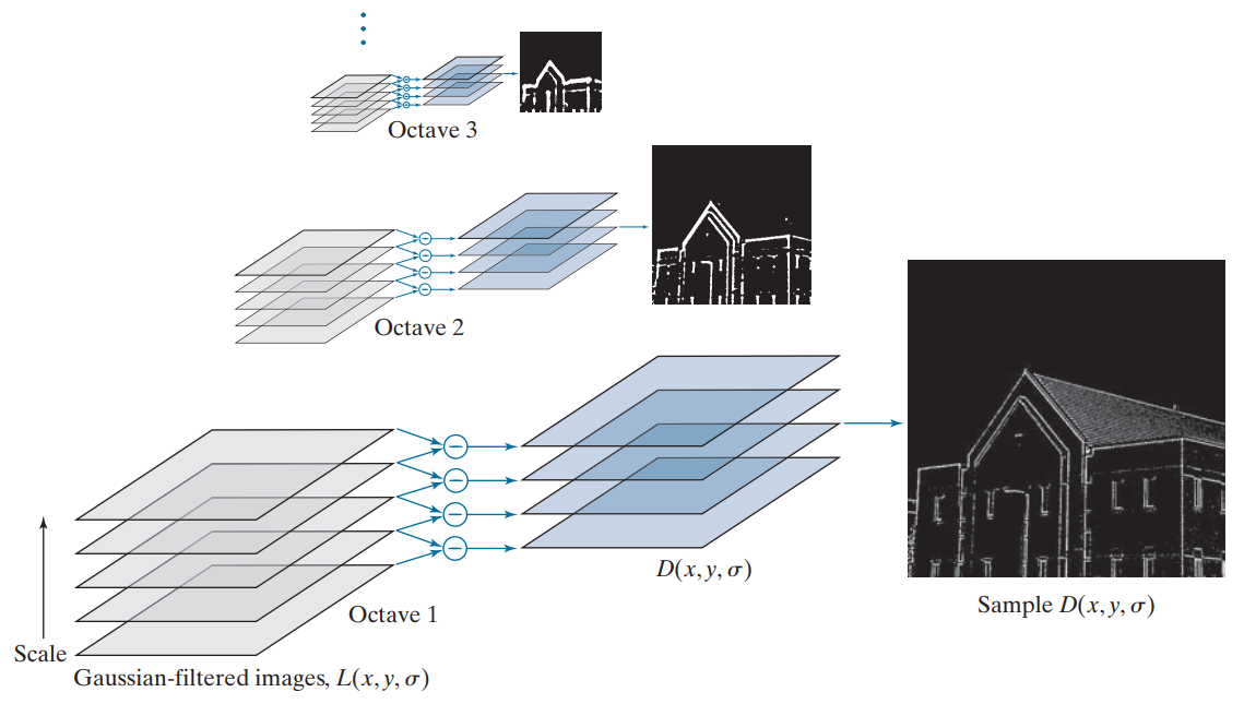
After blurring images, the algorithm subtracts one blurred image from another, producing the Difference of Gaussians (DoG) images to identify keypoints. These highlight regions where pixel intensity changes significantly. These changes are potential keypoints. DoG is computed by subtracting two gaussian-blurred images at different scales using the formula:

D(x,y,σ)=L(x,y,kσ)−L(x,y,σ)

Where 𝑘 is a constant scaling factor.

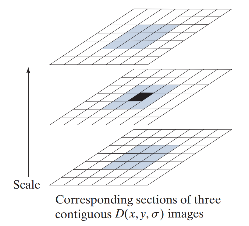
Lastly, the algorithm identifies keypoints by finding maxima and minima also known as local extrema (either very bright or very dark spots) over scale and space in the DoG images. The process is illustrated in the image below. For each pixel in a DoG image, the algorithm compares it with:

• 8 neighbors in the same scale (the same blurred image).
• 9 pixels in the scale above (the previous blurred image).
• 9 pixels in the scale below (the next blurred image).

This comparison across scales ensures that the algorithm detects features that appear strong and consistent at a specific scale.

Step 2: Keypoint Localization

After building the scale-space and finding potential keypoints (local maxima or minima in the DoG images), the locations of detected keypoints need to be refined to make sure they are accurate. To get a more precise location for each keypoint, a mathematical method called a Taylor series expansion is used. Think of it as a way to zoom in and find the exact point where the keypoint should be, like adjusting the focus of a camera for a sharper image.

The Taylor series expansion is used to approximate a function near a given point. In the context of the SIFT algorithm, it's applied to approximate the DoG function around a potential keypoint to refine its location and scale. The Taylor expansion of the DoG function, D(x,y,σ) around a candidate keypoint is given by:

Some keypoints might be located in areas that are too flat or don't have enough variation in brightness (low contrast). These keypoints are not useful because they can be easily affected by noise. Therefore, the intensity (brightness) of each keypoint is checked. If the intensity is below a certain value (0.03, according to the SIFT paper), that keypoint is discarded. This means that only keypoints that are both well-located and have enough contrast are kept. In OpenCV, this threshold for intensity is called contrastThreshold, and it helps ensure that only the best, most stable keypoints are used.

DoG has strong responses along edges, but these points are not reliable. To filter these out, the algorithm checks how well the keypoints are defined by looking at the curvature of the image in different directions. For example, imagine a ridge in a mountain. Along the ridge, the shape doesn’t change much (low curvature), but across the ridge (up or down the mountain), the shape changes a lot (high curvature). If a keypoint behaves like this, where the curvature in one direction is much stronger than in another, it discards it because it's not well-localized.

After filtering out low-contrast and edge-response keypoints, the remaining keypoints are considered as well-localized and stable keypoints, making them ideal for use in further processing.

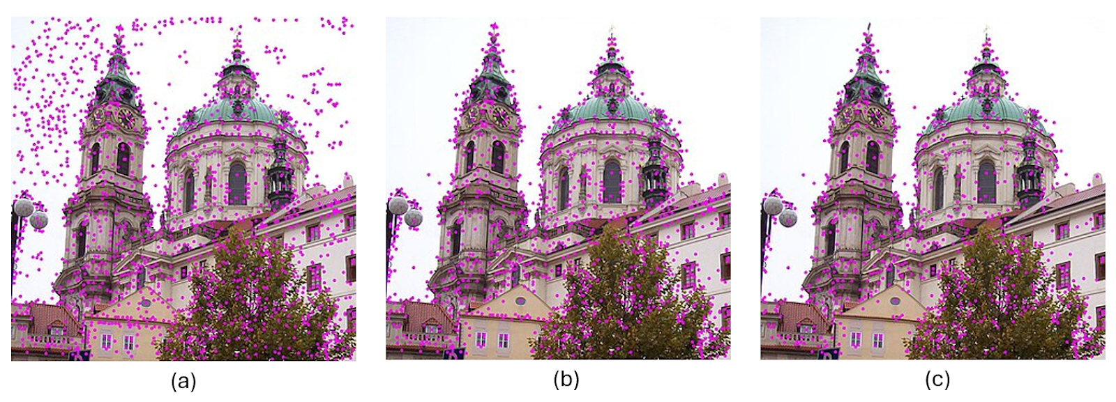
In the above images, first image (a) shows detected keypoints at different scales. The SIFT algorithm removes keypoints that have low contrast (the remaining keypoints are shown in the second image (b)). Then, it further removes keypoints that are located on edges. The final set of keypoints is shown in the last image (c).

Step #3: Orientation Assignment

Now, the identified keypoints are considered stable (they won’t change much if the image is modified slightly). To make these keypoints invariant to rotation, a direction or orientation is given. This helps the algorithm understand that if the image is rotated, it can still find the keypoint in the same spot because it knows which way it’s pointing. This is important because, without it, the keypoint wouldn’t be able to handle rotated images well. 

Each keypoint is given a direction to make the algorithm resistant to image rotation. A small region around the keypoint is analyzed based on its scale, and the magnitude and gradients in the image are calculated. An orientation histogram with 36 bins is created, covering all possible directions (360 degrees). The highest peak in the histogram represents the main direction, but any other peak that is 80% or more of the highest peak is also used to assign an additional direction. This means that keypoints at the same location and scale can have different directions, improving the reliability of matching across images.

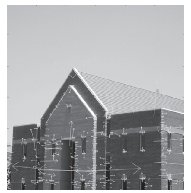
The above image shows keypoints and their directions (indicated by gray arrows) for the entire building. 

Step 4: Keypoint Descriptor

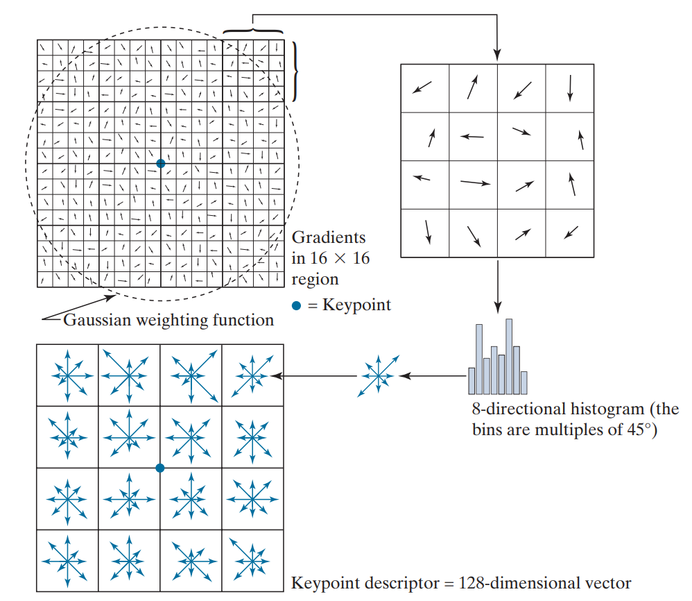
After the keypoints have been detected and assigned an orientation, the next step is to create a descriptor for each keypoint. This descriptor is a compact representation of the keypoint, capturing the local image information around it.

A keypoint descriptor is a way to describe keypoints in an image. To create it, we look at a 16x16 area around each keypoint and divide this area into 16 smaller blocks, each 4x4 in size. For each small block, we create an 8-bin histogram to capture the directions of features. This results in a total of 128 values that make up the keypoint descriptor. The descriptor is scale-invariant, rotation-invariant, and robust to changes in lighting and viewpoint.

SIFT Implementation

Now, let’s see how we can use SIFT. SIFT is now included in the main repository of OpenCV library. The OpenCV provides various functions to implement the SIFT algorithm.

Use the accompanying notebook while reading this blog post to follow along with the examples.

The following steps are used to implement it:

• Initializes a SIFT detector object using SIFT_create() function.
• Detects keypoints in an image using detect() function.
• Draws keypoints on an image using drawKeypoints() function.

Example:

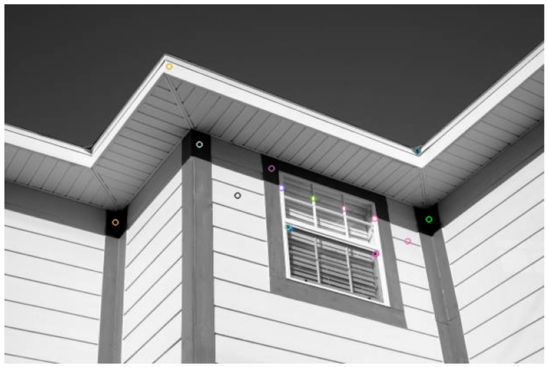
# Load the image
img = cv.imread('house.jpg')
gray = cv.cvtColor(img, cv.COLOR_BGR2GRAY)

# Initialize SIFT detector
sift = cv.SIFT_create()

# Detect keypoints
kp = sift.detect(gray, None)

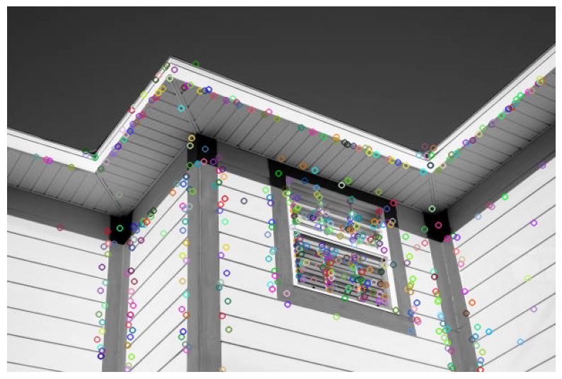
# Draw keypoints on the image
img_with_kp = cv.drawKeypoints(gray, kp, img)

Output:

Detecting keypoints in ROI

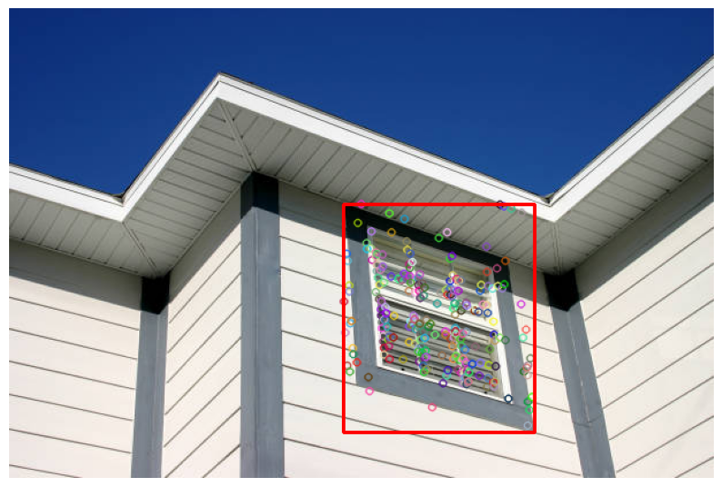
In the above code the second argument to detect() function is the mask that we have defined as None (meaning no mask). However, you can specify mask to limit the area where keypoints are detected. The mask is a binary image where non-zero values indicate the region of interest (ROI) where keypoints should be detected. To detect the keypoint only in the ROI you follow the steps below:

• Create a Mask: You define a mask with the same dimensions as your grayscale image. In this example, the mask is initially all zeros (black), and we set a rectangular region to 255 (white) to specify where we want keypoints to be detected.
• Apply the Mask: Pass the mask as the second argument to the detect() function. Keypoints will only be detected in the white region of the mask.

I our example below, we set a ROI for displaying keypoints only in the area of the image from pixel (290, 170) to (456, 368). This is the area where you see ‘a window’ in the image.  We also draw a rectangle in the output image specifying our ROI.

# Create a mask: initialize with zeros (black)
mask = np.zeros(gray.shape, dtype=np.uint8)

# Define ROI coordinates
x_start, y_start = 290, 170
x_end, y_end = 456, 368

# Set the ROI in the mask to white (255)
mask[y_start:y_end, x_start:x_end] = 255

# Initialize SIFT detector
sift = cv.SIFT_create()

# Detect keypoints using the mask
kp = sift.detect(gray, mask)

# Draw keypoints on the image
img_with_kp = cv.drawKeypoints(img, kp, None)

# Highlight the ROI with a rectangle (in red for visibility)
cv.rectangle(img_with_kp, (x_start, y_start), (x_end, y_end), (0, 0, 255), 2)  # Red rectangle, thickness=2

The following output will be generated.

Parameters of SIFT_create()

The SIFT_create() function also allows us to set the different values to parameters that it accepts to override the default values. These flags are following:

Syntax:

SIFT_create(nfeatures=0, nOctaveLayers=3, contrastThreshold=0.04, edgeThreshold=10, sigma=1.6)

• nfeatures (default: 0): It specifies number of best keypoints to retain. If this value is set to 0, all keypoints detected by the algorithm will be kept. Use if you only need a certain number of keypoints (e.g., for performance reasons), you can set a limit using this parameter.
• nOctaveLayers (default: 3): It specifies the number of layers in each octave. Increasing this number may increase the detection of keypoints at different scales, but it also increases computational cost. A higher value will increase the accuracy at different scales but slow down the algorithm. Please note that it does not effect number of octaves at each layer as it is automatically calculated.
• contrastThreshold (default: 0.04): The contrast threshold is used to filter out weak keypoints. Keypoints with lower contrast are likely to be noise, so they are discarded. Decreasing this value will allow weaker keypoints to be kept, but it may also increase noise in the keypoints. Lower this value to detect more keypoints in low-contrast images, but this might result in more noise.
• edgeThreshold (default: 10): This parameter filters out keypoints that are sensitive to edge-like structures, which can lead to unstable keypoints. A higher value allows more edge-like keypoints, while a lower value excludes them. Increase this value to detect more keypoints along edges but be aware that this might result in less stable keypoints.
• sigma (default: 1.6):  The sigma value used in the Gaussian filter applied to the input image at the first octave. This value affects the scale at which keypoints are detected. This can suppress fine details and noise, potentially leading to more stable keypoints. However, it might also cause some smaller features to be missed.

For example, setting up nfeatures=20, the detector will attempt to find and keep up-to the top 20 most prominent keypoints based on their strength. Please note that sometime you may not see the exact number of specified keypoints.

Example:

# Initialize SIFT detector
sift = cv.SIFT_create(nfeatures=20)

Output:

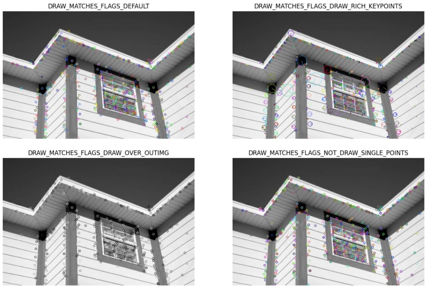
Setting FLAGS for keypoints

The drawKeypoints() function also supports various flags as a fourth argument to visualize keypoints with different styles. These flags are following:

• cv.DRAW_MATCHES_FLAGS_DEFAULT: Draws keypoints with simple circles.
• cv.DRAW_MATCHES_FLAGS_DRAW_RICH_KEYPOINTS: Draws keypoints with size and orientation, making keypoints richer (useful for blob detection).
• cv.DRAW_MATCHES_FLAGS_DRAW_OVER_OUTIMG: Draws keypoints on an output image, leaving the original image unchanged.
• cv.DRAW_MATCHES_FLAGS_NOT_DRAW_SINGLE_POINTS: Draws only keypoints that are part of matching pairs (often used when drawing matches between two images).

Example:

# Initialize SIFT detector
sift = cv.SIFT_create()
kp = sift.detect(gray, None)

# Define different flags to be used for drawing keypoints
flags = [
    cv.DRAW_MATCHES_FLAGS_DEFAULT,
    cv.DRAW_MATCHES_FLAGS_DRAW_RICH_KEYPOINTS,
    cv.DRAW_MATCHES_FLAGS_DRAW_OVER_OUTIMG,
    cv.DRAW_MATCHES_FLAGS_NOT_DRAW_SINGLE_POINTS
]

# Titles corresponding to the flags
flag_titles = [
    "DRAW_MATCHES_FLAGS_DEFAULT",
    "DRAW_MATCHES_FLAGS_DRAW_RICH_KEYPOINTS",
    "DRAW_MATCHES_FLAGS_DRAW_OVER_OUTIMG",
    "DRAW_MATCHES_FLAGS_NOT_DRAW_SINGLE_POINTS"
]

# Plot the images with keypoints using different flags
plt.figure(figsize=(15, 15))
for i, flag in enumerate(flags):
    # Draw keypoints on the image using the current flag
    img_with_kp = cv.drawKeypoints(gray, kp, gray, flags=flag)
    
    # Convert the image from BGR to RGB for displaying with matplotlib
    img_with_kp_rgb = cv.cvtColor(img_with_kp, cv.COLOR_BGR2RGB)

Output:

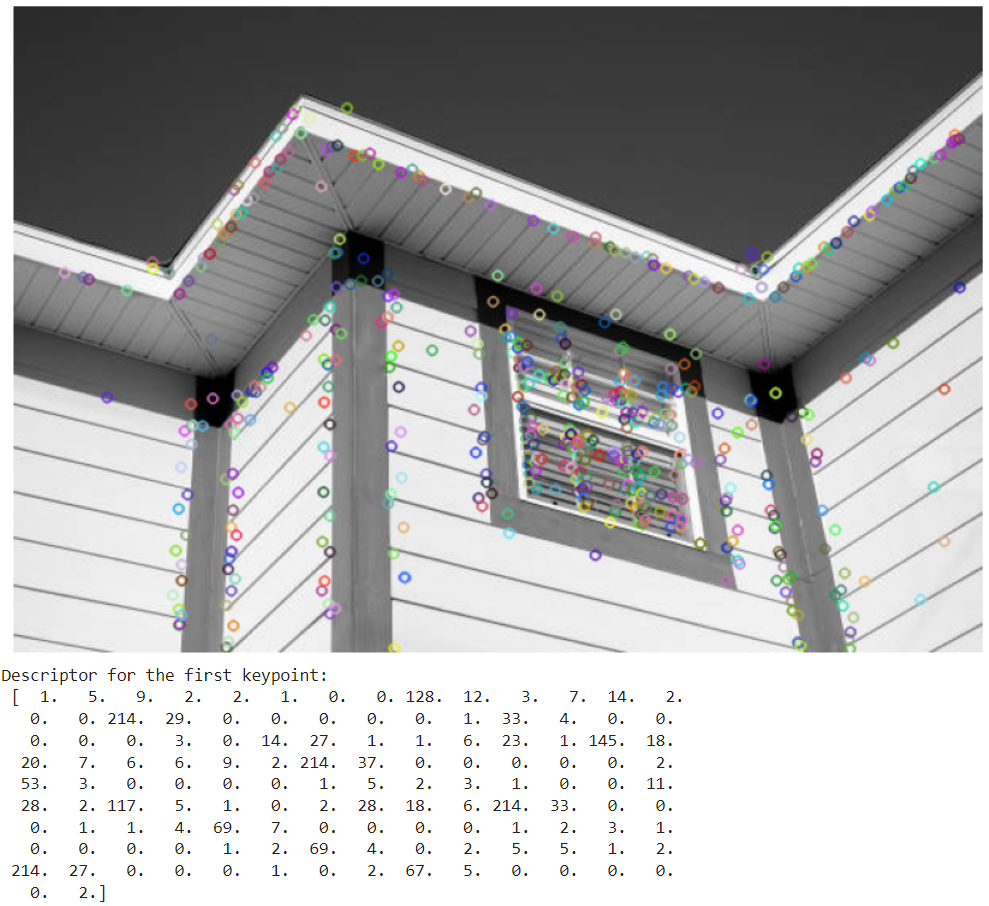
Detecting descriptor

Descriptors are numerical representations of the local image patches around each keypoint, which help in matching keypoints across images. It captures the essential characteristics (such as texture, intensity gradients, and patterns) of the image in the region around the keypoint in a way that is invariant to scale, rotation, and, to some extent, lighting changes.

In the context of feature detection algorithms like SIFT, descriptors are used to uniquely describe each keypoint and help in matching keypoints between different images. The descriptor itself is usually a 128-dimensional vector in SIFT, but this size may vary for other algorithms. 

The compute() function in OpenCV is used to calculate the descriptors for a given set of keypoints detected in an image. You use the compute() function when you have already detected the keypoints in an image using detect(), but have not computed the descriptors yet.

Example:

# Initialize SIFT detector
sift = cv.SIFT_create()

# Detect keypoints (without descriptors)
keypoints = sift.detect(gray, None)

# Compute descriptors for the detected keypoints
keypoints, descriptors = sift.compute(gray, keypoints)

# Draw the keypoints on the image
img_with_keypoints = cv.drawKeypoints(gray, keypoints, img)

...
# Print some descriptors
print("Descriptor for the first keypoint:\n", descriptors[0])

Output:

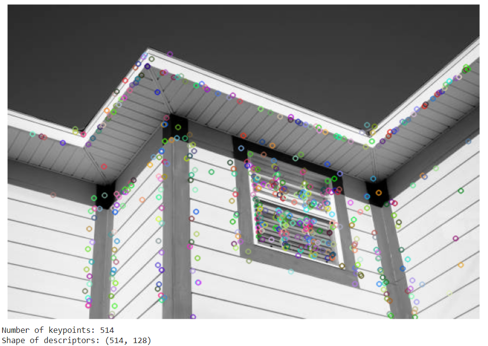
Alternatively you can also use detectAndCompute() function which combines both detection of keypoints and computation of descriptors in a single function call instead of using detect() and compute() functions separately. 

Example:

# Initialize SIFT detector
sift = cv.SIFT_create()

# Detect keypoints and compute descriptors
keypoints, descriptors = sift.detectAndCompute(gray, None)

# Draw keypoints on the image
img_with_kp = cv.drawKeypoints(gray, keypoints, None)

# Convert the image from BGR to RGB for displaying with matplotlib
img_with_kp_rgb = cv.cvtColor(img_with_kp, cv.COLOR_BGR2RGB)

Output:

Application of SIFT: Finding Object

SIFT algorithm is widely used in various applications, including object detection and recognition, image stitching, image retrieval, motion tracking and 3D modeling etc. In this example we will build an application using SIFT to find an object in another image. The application will return a JSON response indicating PASS or FAIL based on the number of keypoints detected (i.e. >=100 keypoints), along with the number of detected keypoints. It will also visualize the results. 

Example:

# Initialize SIFT detector
sift = cv.SIFT_create()

# Find keypoints and descriptors
kp1, des1 = sift.detectAndCompute(object_img, None)
kp2, des2 = sift.detectAndCompute(scene_img, None)

# FLANN parameters
FLANN_INDEX_KDTREE = 1
index_params = dict(algorithm=FLANN_INDEX_KDTREE, trees=5)
search_params = dict(checks=50)

# FLANN-based matcher
flann = cv.FlannBasedMatcher(index_params, search_params)
matches = flann.knnMatch(des1, des2, k=2)

# Store good matches using Lowe's ratio test
good_matches = []
for m, n in matches:
    if m.distance < 0.7 * n.distance:
        good_matches.append(m)

# Prepare result
num_keypoints = len(good_matches)
result = {
    "status": "PASS" if num_keypoints >= min_keypoints else "FAIL",
    "keypoints_detected": num_keypoints
}

# Visualize results
img_matches = cv.drawMatches(object_img, kp1, scene_img, kp2, good_matches, None, flags=cv.DrawMatchesFlags_NOT_DRAW_SINGLE_POINTS)

Output:

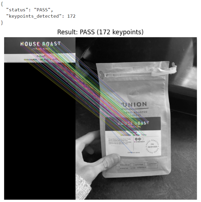
This example application aims to find corresponding points between the ‘label’ image and ‘coffee package’ image. FLANN is used for efficient matching, and Lowe's ratio test (as described in this paper) helps to ensure that only strong, unique matches are considered. The number of good matches determines whether the object is considered found (PASS) or not (FAIL) in the scene.

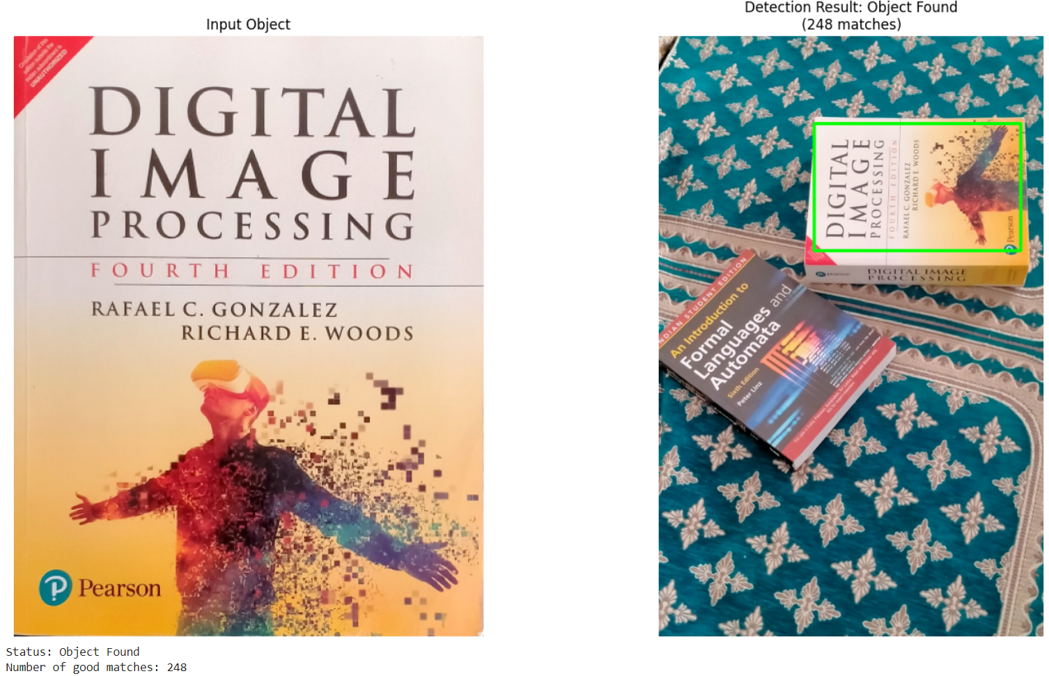
Here's another example. In this example we perform object detection and draw a bounding box for the detected object, regardless of its orientation in the search image. Please find the code for the below output in accompanying notebook.

Output:

Conclusion

In this blog post, we explored the SIFT algorithm in detail, discussing how it works and how to implement it using the OpenCV library. Additionally, Roboflow offers a no-code solution for applying this powerful algorithm. For further insights, I recommend checking out the post How to Use Scale-Invariant Feature Transform (SIFT) to learn more.