
Object detection is a computer vision task that involves identifying and localizing objects within an image or video. It not only classifies objects present in the image but also provides their locations, typically by drawing bounding boxes around them.
Object detection metrics evaluate how well an object detection model detects and localizes objects in an image. Here are some of the key metrics that we will discuss in this blog:
- Intersection over Union (IoU)
- Precision
- Recall
- Average Precision (AP)
- Mean Average Precision (mAP)
- F1 Score
Why Do Object Detection Metrics Metrics Matter?
Model Evaluation: These metrics provide a quantitative way to evaluate the performance of object detection models. They help in comparing different models and selecting the best one for a given task.
Error Analysis: By analyzing precision, recall, and IoU, developers can identify specific areas where the model is performing poorly. For example, low recall might indicate that the model is missing many objects, while low precision might indicate a high number of false positives.
Optimization: Metrics like mAP and F1 score guide the optimization process. Developers can fine-tune their models to improve these metrics, leading to better overall performance.
Benchmarking: Standard metrics allow for fair benchmarking of different models and approaches. This is crucial in research and development, where new techniques are constantly being proposed and evaluated.
Real-world Application: In practical applications, such as autonomous driving, surveillance, and medical imaging, accurate object detection is critical. Reliable metrics ensure that the models deployed in these applications meet the required performance standards.
Object detection metrics are essential for evaluating, optimizing, and benchmarking models. They provide insights into the strengths and weaknesses of the models, guiding improvements and ensuring reliable performance in real-world applications.
Key Terms in Object Detection Metrics
In the context of object detection, the terms True Positives (TP), True Negatives (TN), False Positives (FP), and False Negatives (FN) are used to evaluate the performance of a model. Let's understand each of these concepts in the context of an object detection model that identifies and localizes cats in images.
True Positives (TP)
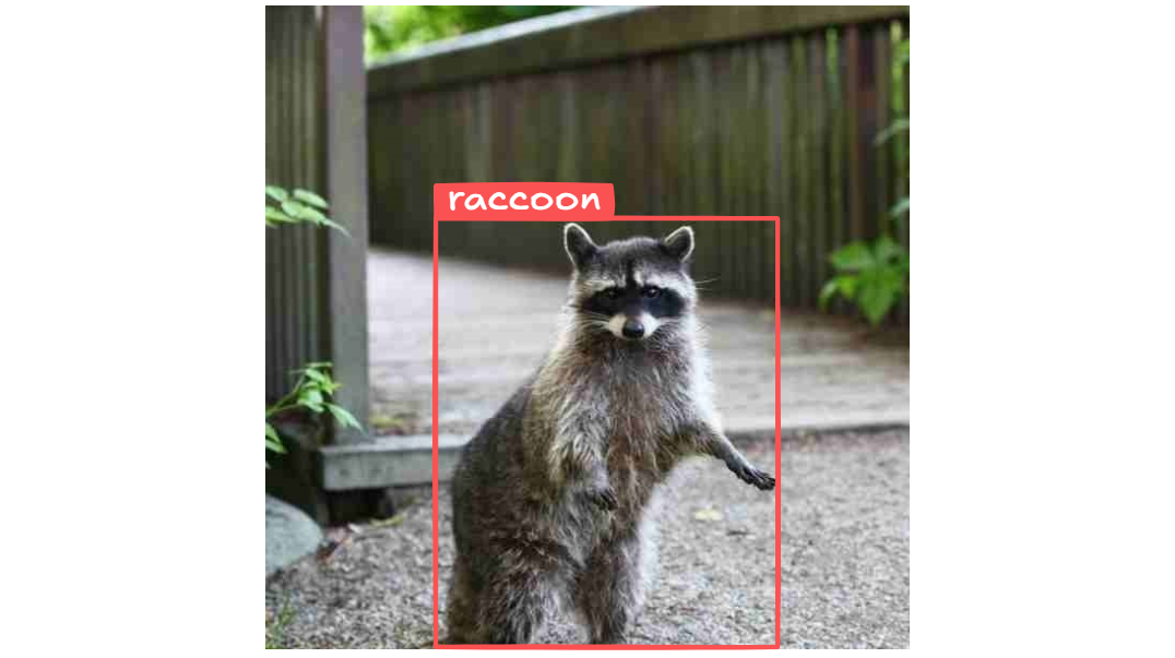
True Positives occur when the model correctly identifies and localizes an object of interest. In this context, it means the model accurately detects and draws a bounding box around a raccoon in the image.
Example
- Scenario: Detecting raccoon in an image.
- Case: An image contains a raccoon, and the model correctly identifies it as a raccoon and draws a bounding box around it.
- Outcome: True Positive for the raccoon class.
True Negatives (TN)
True Negatives occur when the model correctly identifies that an object of interest is not present. In this context, it means the model correctly determines that there is no cat in the image.
Example
- Scenario: Detecting raccoon in image.
- Case: An image does not contain a raccoon, and the model correctly identifies that there are no raccoon. The model does not draw any bounding boxes for cats.
- Outcome: True Negative for cat class.
False Positives (FP)
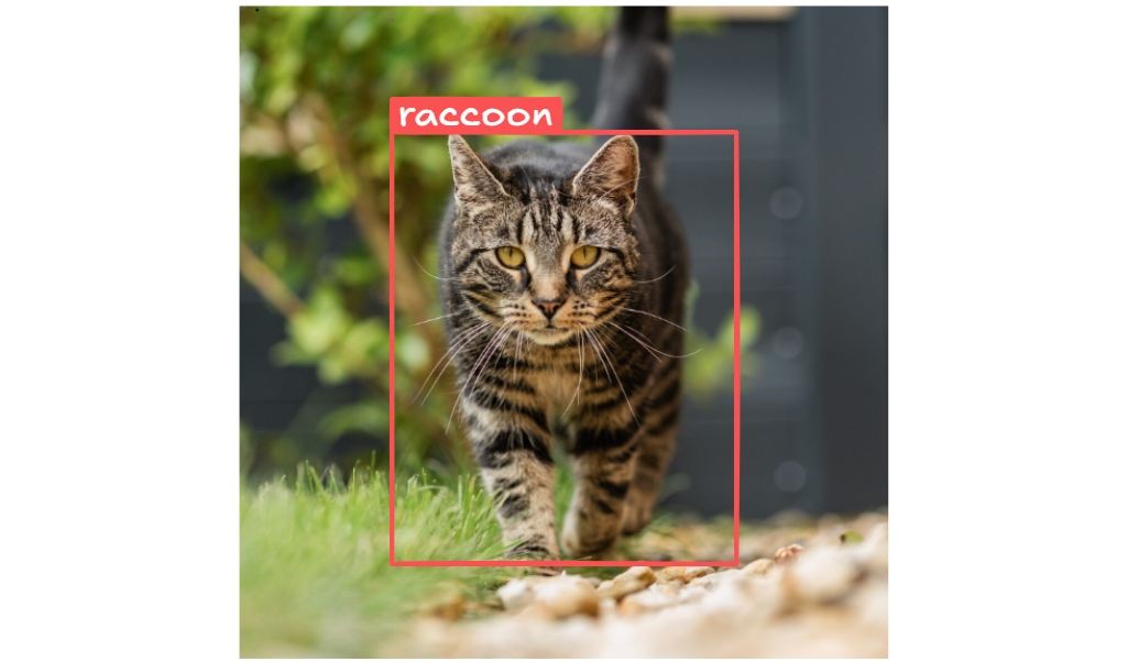
False Positives occur when the model incorrectly identifies an object of interest where there is none. In this context, it means the model identifies a raccoon in the image when there is not a raccoon.
Example
- Scenario: Detecting raccoon in image.
- Case: An image does not contain a raccoon, but the model incorrectly identifies a raccoon and draws a bounding box around a non-raccoon object (i.e. cat).
- Outcome: False Positive for the raccoon class.
False Negatives (FN)
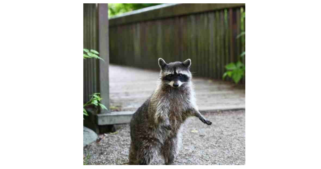
False Negatives occur when the model fails to identify an object of interest that is present. In this context, it means the model misses a raccoon in the image.
Example
- Scenario: Detecting raccoon in images.
- Case: An image contains a raccoon, but the model fails to identify it and does not draw a bounding box around it.
- Outcome: False Negative for the cat class.
Confidence Score
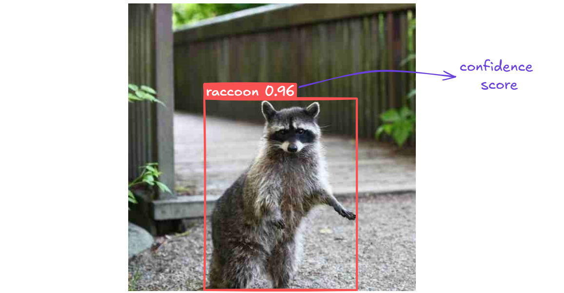
A confidence score is a value, typically between 0 and 1, that quantifies the model's confidence in its prediction. A higher confidence score indicates a higher level of certainty, while a lower score indicates less certainty.
In object detection, the model predicts bounding boxes around objects in an image and assigns a confidence score to each prediction. This score reflects the model's confidence that the detected object is correctly identified and localized.
For example, if the model detects a raccoon in an image with a confidence score of 0.96, it means the model is 96% confident that the detected object is indeed a raccoon.
The object detection model calculates the confidence score by multiplying the probability that an object exists in a predicted box (objectness score) with the probability that the object belongs to a specific class (class score). These probabilities are learned during training using a loss function that penalizes incorrect detections and classifications. For each predicted box it is calculated as:

Where:
- 𝜎(𝑡𝑜) - Sigmoid of objectness logit, outputs between 0 and 1.
- Softmax(𝑡𝑐) - Probability that the object belongs to class c.
Key Object Detection Metrics
Let's delve into each of the object detection metrics, their formulas, and examples of how to calculate them. We'll also note any dependencies between the metrics.
Intersection over Union (IoU)
IoU is a measure of the overlap between the predicted bounding box and the ground truth bounding box. It is calculated as the area of overlap divided by the area of union of the two boxes.

Where
- Area of overlap is the region where the predicted bounding box and the ground truth bounding box intersect (i.e., the shared area between both boxes).
- Area of union is the total area covered by both the predicted and ground truth boxes combined, without double-counting the overlap.
Thus, we can define IoU as the ratio of the overlapping area between a predicted box Bpred and the ground‑truth box Bgt to the area of their union.

IoU can be calculated with following steps.
Step #1: Get coordinates of both boxes
Ground Truth Box:𝑥_𝑔𝑡1, 𝑦_𝑔𝑡1, 𝑥_𝑔𝑡2, 𝑦_𝑔𝑡2
(Top-left and bottom-right corners of the actual object)
Predicted Box:𝑥_𝑝1, 𝑦_𝑝1, 𝑥_𝑝2, 𝑦_𝑝2
(Top-left and bottom-right corners of the model's prediction)
Step #2: Find the overlapping area (intersection)
Top-left of intersection:𝑥𝐴 = max(𝑥_𝑔𝑡1, 𝑥_𝑝1)
𝑦𝐴 = max(𝑦_𝑔𝑡1, 𝑦_𝑝1)
Bottom-right of intersection:𝑥𝐵 = min(𝑥_𝑔𝑡2, 𝑥_𝑝2)
𝑦𝐵 = min(𝑦_𝑔𝑡2, 𝑦_𝑝2)
Step #3: Calculate intersection area
inter_area = max(0,𝑥𝐵−𝑥𝐴) × max(0,𝑦𝐵−𝑦𝐴)
(This is the width × height of the overlapping region)
Step #4: Calculate area of each box
Ground truth area:area_gt = (𝑥_𝑔𝑡2−𝑥_𝑔𝑡1) × (𝑦_𝑔𝑡2−𝑦_𝑔𝑡1)
Predicted box area:area_pred = (𝑥_𝑝2−𝑥_𝑝1) × (𝑦_𝑝2−𝑦_𝑝1)
Step #5: Calculate the union area
union_area = area_gt + area_pred − inter_area
(This includes both areas, but subtracts the overlapping part so it's not counted twice)
Step #6: Calculate IoU
IoU = inter_area / union_area
This gives a score between 0 and 1:
- 0 = no overlap
- 1 = perfect overlap
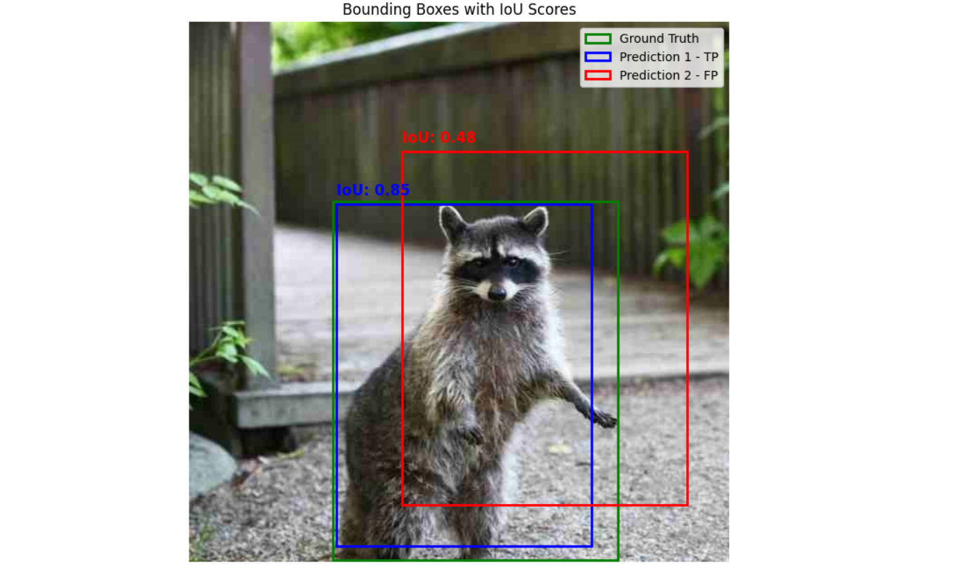
Now let’s see an example. Suppose we have following data.
image_name = "raccoon_1.jpg"
gt_box = [159, 199, 476, 598]  # Ground truth box
pred_boxes = [
    [163, 202, 447, 582],  # TP
    [236, 144, 553, 536]   # FP
]
We define the following function to calculate the IoU.
def compute_iou(box1, box2):
    xA = max(box1[0], box2[0])
    yA = max(box1[1], box2[1])
    xB = min(box1[2], box2[2])
    yB = min(box1[3], box2[3])

    inter_area = max(0, xB - xA) * max(0, yB - yA)
    box1_area = (box1[2] - box1[0]) * (box1[3] - box1[1])
    box2_area = (box2[2] - box2[0]) * (box2[3] - box2[1])

    union_area = box1_area + box2_area - inter_area
    return inter_area / union_area if union_area != 0 else 0
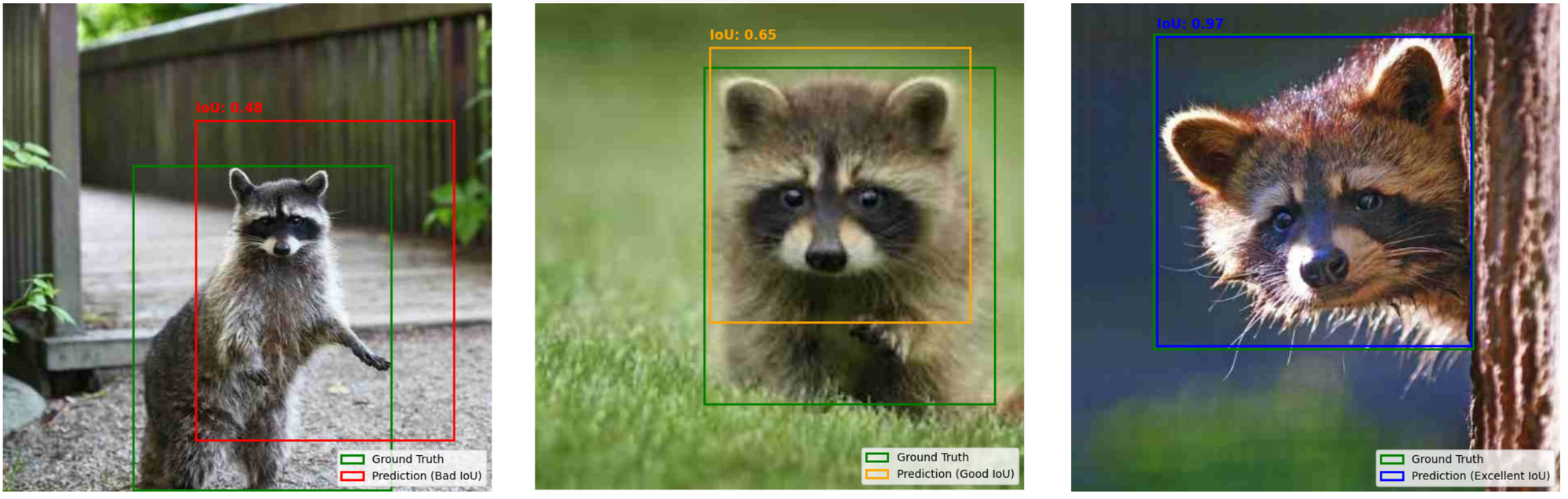
Now that we understand what Intersection over Union (IoU) is and how it's calculated, the next question is what constitutes a good IoU score? IoU scores typically range from 0.0 to 1.0, where
- IoU = 0.0 means no overlap between the predicted and ground truth boxes.
- IoU = 1.0 means a perfect match, the boxes align exactly.
But most real-world predictions fall somewhere in between. Here's a general guideline:
| IoU Score | Quality | Interpretation |
| 0.00 – 0.30 | Bad | Very little overlap, the prediction poorly matches the actual object |
| 0.31 – 0.60 | Good | Some overlap, the object is partially detected, but localization needs improvement |
| 0.61 – 1.00 | Excellent | Strong overlap, the predicted box tightly fits the ground truth, showing high precision |
Let’s see how to classify bad, good and excellent IoU. Consider following data for this example.
image_data = {
    "raccoon_1.jpg": {
        "gt": [159, 199, 476, 598],
        "preds": [
            [236, 144, 553, 536]   # FP
        ]
    },
    "raccoon_2.jpg": {
        "gt": [207, 81, 563, 494],
        "preds": [
            [214, 57, 533, 394]     # FP
        ]
    },
    "raccoon_3.jpg": {
        "gt": [101, 37, 492, 424],
        "preds": [
            [105, 40, 490, 420]    # TP
        ]
    }
}
Running the code provided in example notebook will give you following outputs.
In practice, most object detectors aim for IoU ≥ 0.5 to count as a true positive. This classification is critical because IoU is the core criterion for deciding whether a detected object is considered a true positive. For example, many evaluation protocols like PASCAL VOC consider a prediction correct only if its IoU with the ground truth is at least 0.5.
Using higher thresholds (e.g., 0.75) makes the evaluation stricter, rewarding models that offer more accurate localization. This distinction is especially important in applications like medical imaging or autonomous driving, where precise object boundaries can significantly impact downstream decisions. Understanding IoU quality helps developers:
- Tune detection models for stricter or looser localization.
- Set appropriate thresholds for accepting predictions.
- Interpret whether a model is merely detecting an object or accurately pinpointing it.
Precision
Precision measures how accurate your model’s positive predictions are. In simpler terms, it answers the question:
"Out of all objects that my model detected, how many are actually correct?"
Precision directly relates to the concept of False Positives (FP), or "incorrect detections," and True Positives (TP), or "correct detections." Mathematically, precision is defined as:

Why is IoU Required in Precision?
In object detection, a True Positive (TP) is not just about correctly predicting the class of an object. The predicted box must also be accurately placed. IoU is the standard metric used to measure this accuracy of placement.
Precision depends on counting how many detections are correct (TP) and how many are incorrect (FP). But how do you decide if a detection is correct or incorrect? You use IoU to set a threshold.
- If IoU ≥ threshold (commonly 0.5), the prediction counts as a True Positive (correct detection).
- If IoU < threshold, it counts as a False Positive (incorrect detection).
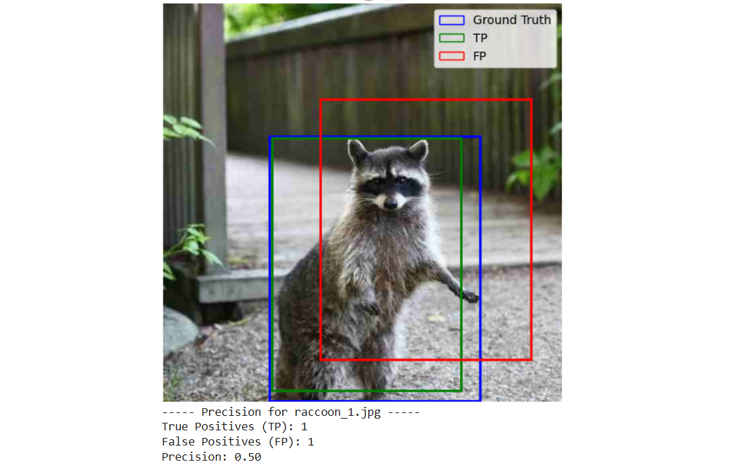
Thus, without IoU, you can't precisely differentiate a good bounding box from a bad bounding box. IoU acts as the gatekeeper, determining whether each prediction is considered accurate enough. To understand this let’s imagine you have following image data with ground truth and prediction from model.
image_name = "raccoon_1.jpg"
gt_box = [159, 199, 476, 598]
pred_boxes = [
     [163, 202, 447, 582],      # TP
     [236, 144, 553, 536]       # FP
]
You calculate precision with following steps.
Step #1: Set an IoU threshold, commonly 0.5.
Step #2: Match predicted boxes with ground truth boxes. A predicted box is a True Positive (TP) if it has IoU ≥ threshold with any unmatched ground truth box. A predicted box is a False Positive (FP) if IoU < threshold, or it matches a ground truth box that is already matched.
Step #3: Count TP and FP where TP is the number of correct predictions and FP is the number of incorrect predictions.
Step #4: Calculate Precision as:
precision = TP / (TP + FP) if (TP + FP) > 0 else 0
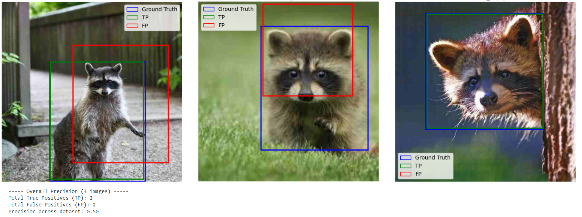
When you execute the code in the notebook to calculate precision for a single image, the following output will be displayed.
For object detection precision can be calculated for both single images and across multiple images. The precision is calculated across multiple images by aggregating true positives (TP) and false positives (FP) from all images. For each image, the ground truth box is compared with predicted boxes using the IoU score. A prediction is considered a true positive if its IoU with the ground truth is greater than or equal to a threshold (0.5) and the ground truth hasn't been matched yet; otherwise, it is counted as a false positive. This process is repeated for every image, and the total TP and FP are summed up. Finally, overall precision is calculated using the formula:

giving a single precision score for the entire dataset. Running the code provided in notebook to calculate precision on multiple images should give you the following output.
Recall
Recall measures how good the model is at finding all existing objects in images. In simpler terms, recall answers the following question:
"Out of all actual objects present in an image (ground truths), how many did my model successfully detect?"
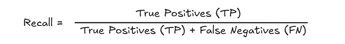
Recall focuses on False Negatives (FN), which occur when your model fails to detect an object that truly exists in the image. Mathematically, recall is defined as:
Why is IoU Required in Recall?
For object detection model, Recall measures how many of the actual objects your model successfully finds. But before you can count a detection as a “hit,” you need a way to decide whether a predicted box really corresponds to a ground-truth box. That’s exactly what IoU does. It defines a True Positive for Recall. Without IoU you’d have no systematic way to say “this prediction matches that ground truth.” With IoU, you set a threshold (commonly 0.5) that
- If a predicted box’s IoU with a ground-truth box ≥ 0.5, you count it as a True Positive (TP).
- If no prediction reaches that overlap threshold for a given ground truth, that object becomes a False Negative (FN).
Because recall = TP / (TP + FN), how you define TP directly drives your recall score.
Here’s the output of recall calculation on single image from the example given in notebook.
Calculating recall for multiple images in object detection follows a similar approach to calculating precision. Recall measures the ability of the model to identify all relevant instances of a particular class. The recall is calculated across multiple images by counting how many ground truth boxes are correctly detected (true positives) and how many are missed (false negatives). For each image, every ground truth box is compared with all predicted boxes using the IoU score. If a predicted box has IoU ≥ threshold (0.5) and hasn't been used already, it is considered a true positive. If no prediction matches a ground truth box, it is counted as a false negative. This is done for all images, and the total TP and FN are aggregated. Finally, overall recall is calculated using the formula:

giving a single recall score for the entire dataset. Following the output from the code given in the notebook to calculate recall for multiple images.

Here in the second image the FN is 1 because the raccoon is in the image, but model did not detect it.
Average Precision
Average Precision (AP) is a key metric used to evaluate the performance of object detection models. It provides a single value that summarizes the precision-recall curve (an area under a class’s Precision‑Recall curve). It turns the whole curve, which shows how precision falls as recall rises when you lower the confidence threshold, into a single number between 0 and 1 (or 0–100 %). High AP means the detector can keep precision high while recovering most objects. It offers a comprehensive measure of the model's accuracy and reliability.
The general formula for VOC-style (Increasing Recall) interpolated AP is:

Where:
- Ri = Recall at ith point
- Pi = Precision at ith point
- (Ri−Ri−1) = Change in recall between consecutive points
This means, for every increase in recall, we calculate the area under the curve by multiplying that increase with the corresponding precision value. In the code example in accompanying notebook, AP is implemented as follows:
def compute_ap(recalls, precisions):
    # Create a dictionary to store the maximum precision for each recall value
    pr_dict = {}
    for r, p in zip(recalls, precisions):
        if r not in pr_dict or p > pr_dict[r]:
            pr_dict[r] = p

    # Sort recall values in ascending order (increasing)
    sorted_recalls = sorted(pr_dict.keys())
    sorted_precisions = [pr_dict[r] for r in sorted_recalls]

    # Add recall=0.0 with maximum precision if not present
    if 0.0 not in pr_dict:
        # Insert at beginning
        sorted_recalls.insert(0, 0.0)
        # Use the maximum precision as the interpolated value at recall=0
        sorted_precisions.insert(0, max(sorted_precisions) if sorted_precisions else 0.0)

    # Apply interpolation (VOC-style)
    for i in range(len(sorted_precisions)-2, -1, -1):
        sorted_precisions[i] = max(sorted_precisions[i], sorted_precisions[i+1])

    # Compute AP using increasing recall formula
    ap = 0.0
    for i in range(1, len(sorted_recalls)):
        delta_r = sorted_recalls[i] - sorted_recalls[i-1]
        ap += delta_r * sorted_precisions[i]

    return ap
What this code does?
- Removes duplicate recall values, keeping only the maximum precision for each unique recall.
- Sorts recalls in increasing order.
- Ensures that precision values never decrease as recall increases (VOC interpolation).
- Computes AP as the area under the precision-recall curve using increasing recall method.
Alternatively, AP can also be calculated using decreasing recall method. It is mathematically expressed as:

The following are the steps to calculate Average Precision (AP)
Step #1: Collect predictions and ground truth boxes for all images.
Step #2: Sort predictions by confidence score (descending).
Step #3: Assign TP or FP to each prediction using IoU ≥ threshold (e.g., 0.5).
Step #4: Compute precision and recall for all points.
Step #5: Plot precision-recall curve.
Step #6: Compute AP as the area under this curve.
Mean Average Precision (mAP)
Mean Average Precision (mAP) is the mean (average) of AP values across different classes and/or different IoU thresholds. So mAP is calculated after calculating the AP. It is one of the most common and popular metric used to evaluate object detection models. mAP is used to answer:
“How well does my object detector perform across all classes and object locations?”
mAP can be calculated as:

Where:
- 𝑁 is the number of classes
- 𝐴𝑃𝑖 is the average precision for class
The following two terms are used in mAP.
mAP@50: Meaning Mean Average Precision calculated using an IoU threshold of 0.50. In this, a predicted bounding box is considered correct (True Positive) if its IoU with the ground-truth box is ≥ 0.50. mAP@50 is easier to score high and used in PASCAL VOC benchmarks. It is often referred to as “loose” matching.
mAP@75: Meaning Mean Average Precision calculated using an IoU threshold of 0.75. In this, a predicted bounding box is considered correct (True Positive) if its IoU with the ground-truth box is ≥ 0.75. This threshold is stricter than 0.50, requiring predictions to align more accurately with the ground truth. mAP@75 is commonly used in COCO benchmarks to evaluate the precision of object localization. Since it demands tighter overlaps, models generally score lower on mAP@75 compared to mAP@50. It is often referred to as “tight” matching and better reflects a model's ability to precisely detect object boundaries.
mAP@50:95: Means Mean Average Precision averaged across IoU thresholds from 0.50 to 0.95 (step = 0.05). The IoU thresholds used here is:

Here we use 10 different IoU thresholds. For each class, calculate the Average Precision (AP) at each threshold then average those 10 AP values to get one AP for the class. Finally, average the APs of all classes to get the mean Average Precision (mAP@[.50:.95]). mAP@50:95 is stricter and more realistic and used in COCO benchmark. It requires the detector to be precise (tight bounding boxes).
| Metric | IoU Range | Style | Notes |
| mAP@50 | IoU ≥ 0.50 | VOC-style | Easier; counts loose matches |
| mAP@50 | IoU ≥ 0.70 | COCO-style | Easier; counts tight matches |
| mAP@50:95 | 0.50–0.95 (step 0.05) | COCO-style | Stricter; averages across all IoU levels |
Example of calculating AP and mAP
Now let’s see an example of calculating AP an mAP. Let’s say we have 10 images with three classes (cat, dog, raccoon) and IoU threshold is 0.5. We’ll define:
- Ground truth boxes per image
- Model predictions with confidence scores
- TP/FP labeling using IoU
- AP calculation for each class
- Final mAP
Step #1: Dataset (10 images, 3 classes)
We'll use simplified boxes (abstract numbers), and assume 1 GT box per image.
Ground Truth (GT)
| Image | Class | GT Box |
| image_1.jpg | Cat | [10,10,50,50] |
| image_2.jpg | Dog | [20,20,60,60] |
| image_3.jpg | Raccoon | [30,30,70,70] |
| image_4.jpg | Dog | [15,15,55,55] |
| image_5.jpg | Cat | [25,25,65,65] |
| image_6.jpg | Raccoon | [40,40,80,80] |
| image_7.jpg | Dog | [30,30,70,70] |
| image_8.jpg | Cat | [35,35,75,75] |
| image_9.jpg | Raccoon | [20,20,60,60] |
| image_10.jpg | Dog | [50,50,90,90] |
Predictions (Box + Confidence)
| Image | Predicted Class | Box | Confidence |
| image_1.jpg | Cat | [12,12,48,48] | 0.9 |
| image_2.jpg | Dog | [22,22,58,58] | 0.8 |
| image_3.jpg | Raccoon | [32,32,68,68] | 0.85 |
| image_4.jpg | Dog | [0,0,30,30] | 0.7 (FP) |
| image_5.jpg | Cat | [10,10,30,30] | 0.6 (FP) |
| image_6.jpg | Raccoon | [42,42,78,78] | 0.9 |
| image_7.jpg | Dog | [28,28,68,68] | 0.95 |
| image_8.jpg | Cat | [36,36,76,76] | 0.88 |
| image_9.jpg | Raccoon | [10,10,40,40] | 0.5 (FP) |
| image_10.jpg | Dog | [50,50,90,90] | 0.92 |
Step #2: Label TP and FP using IoU ≥ 0.5
Let’s assume IoU ≥ 0.5 for all correct predictions.
| Image | Class | TP or FP |
| image_1.jpg | Cat | TP |
| image_2.jpg | Dog | TP |
| image_3.jpg | Raccoon | TP |
| image_4.jpg | Dog | FP |
| image_5.jpg | Cat | FP |
| image_6.jpg | Raccoon | TP |
| image_7.jpg | Dog | TP |
| image_8.jpg | Cat | TP |
| image_9.jpg | Raccoon | FP |
| image_10.jpg | Dog | TP |
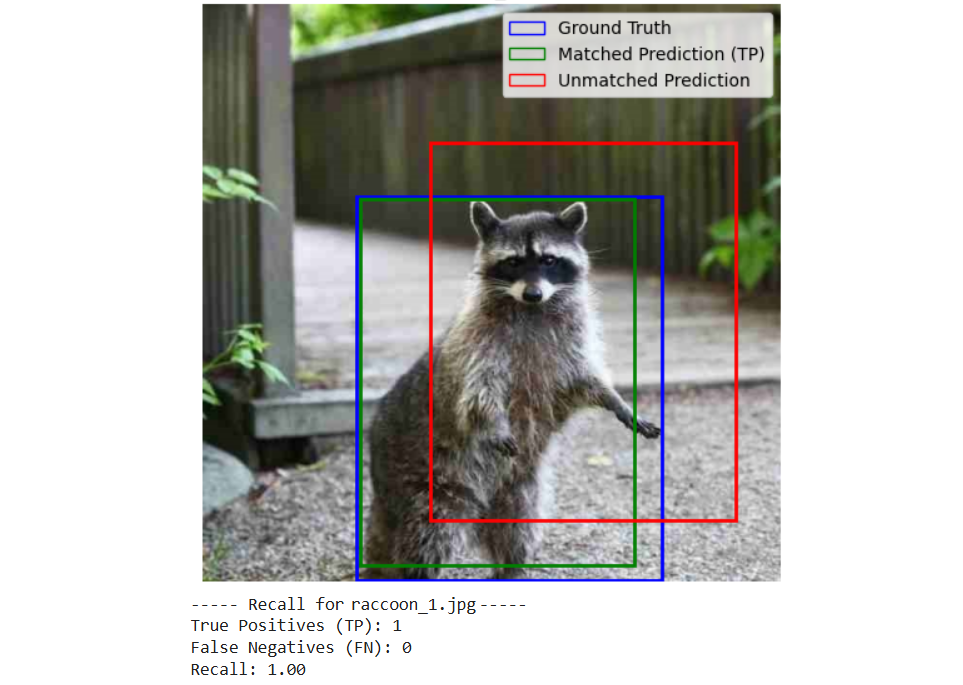
Step #3: Compute AP per class using VOC-style (Increasing Recall)
Class: Cat
Predictions (sorted by confidence):
| Conf | TP/FP |
| 0.9 | TP |
| 0.88 | TP |
| 0.6 | FP |
Precision/Recall:
After 1st: P = 1.00, R = 0.33
After 2nd: P = 1.00, R = 0.67
After 3rd: P = 0.67, R = 0.67
When recall doesn't increase but precision changes, we should select the highest precision for that recall value. So,
AP_Cat = (0.33 × 1.00) + (0.34 × 1.00) = 0.67
There are 3 ground truth objects (total_gt = 3) for class "Cat". Model makes predictions in order of confidence. Therefore,
| Step | Prediction is... | TP | FP | Precision | Recall |
|---|---|---|---|---|---|
| 1 | Correct (TP) | 1 | 0 | 1 / (1 + 0) = 1.00 | 1 / 3 = 0.33 |
| 2 | Correct (TP) | 2 | 0 | 2 / (2 + 0) = 1.00 | 2 / 3 = 0.67 |
| 3 | Incorrect (FP) | 2 | 1 | 2 / (2 + 1) = 0.67 | 2 / 3 = 0.67 |
remember that in recall, TP+FN = total ground truths
Class: Dog
Predictions (sorted by confidence):
| Conf | TP/FP |
| 0.95 | TP |
| 0.92 | TP |
| 0.8 | TP |
| 0.7 | FP |
Precision/Recall:
After 1st: P = 1.00, R = 0.25
After 2nd: P = 1.00, R = 0.50
After 3rd: P = 1.00, R = 0.75
After 4th: P = 0.75, R = 0.75
Since recall does not increase after the 4th prediction, we select the recall that has maximum precision for calculating AP. So,
AP_Dog = (0.25 × 1.00) + (0.25 × 1.00) + (0.25 × 1.00) = 0.75
Class: Raccoon
Predictions (sorted by confidence):
| Conf | TP/FP |
| 0.9 | TP |
| 0.85 | TP |
| 0.5 | FP |
Precision/Recall:
After 1st: P = 1.00, R = 0.33
After 2nd: P = 1.00, R = 0.67
After 3rd: P = 0.67, R = 0.67
Since recall does not increase after the 3rd prediction, we select the recall that has maximum precision for calculating AP. So,
AP_Raccoon = (0.33 × 1.00) + (0.34 × 1.00) = 0.67
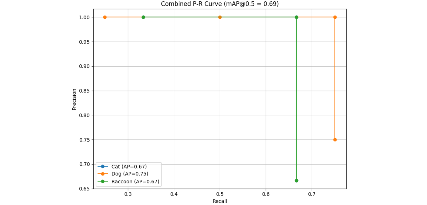
Step #4: Calculate mAP
mAP@0.5 = 0.67 + 0.75 + 0.67 / 3 = 0.69
Therefore
| Class | AP |
| Cat | 0.67 |
| Dog | 0.75 |
| Raccoon | 0.67 |
| mAP | 0.69 |
When you run the code provided in notebook, you will see following output.
F1 Score
F1 Score is the harmonic mean of Precision and Recall, used to evaluate the accuracy of an object detection model in terms of both correctness and completeness. Precision measures how many predicted bounding boxes are actually correct (True Positives), while Recall measures how many of the actual ground truth objects were successfully detected. In object detection, a prediction is typically considered correct if it meets an IoU threshold (such as ≥ 0.50). The F1 Score balances these two metrics and is calculated as:

F1 Score is particularly useful when there is a need to trade-off between false positives and false negatives. A high F1 Score means the model is detecting most objects accurately (high recall) and not predicting too many incorrect boxes (high precision). In this context, the F1 Score is often computed per class at a fixed IoU threshold (like 0.50 or 0.75), helping evaluate how well the model performs for each category. Unlike mAP, which summarizes performance across multiple thresholds or all confidence levels, F1 Score is usually reported at a specific operating point or threshold, offering a focused view of model performance at that point.
Following is the output from the example used to calculate the F1 score in the notebook.

Evaluate Models with Object Detection Metrics
In this blog, we explored the essential metrics used to evaluate object detection models, including IoU, Precision, Recall, Average Precision (AP), Mean Average Precision (mAP), F1 Score. These metrics help us not only understand how well a model performs in terms of correctly identifying and localizing objects but also reveal where and why a model might be failing.
We learned how IoU is the foundation for deciding if a prediction is valid by comparing overlaps between predicted and ground truth bounding boxes. Precision and Recall give us insight into the model’s ability to avoid false alarms and detect all relevant objects, respectively. AP and mAP provide a summary of model performance across different classes and IoU thresholds, offering a balanced and standardized way to benchmark models. The F1 Score helps us balance precision and recall.
Key Object Detection Metrics Takeaways
- IoU is critical for determining true positives in object detection.
- Precision and Recall measure the correctness and completeness of predictions.
- mAP@50 and mAP@50:95 are standard benchmarking scores in object detection, with mAP@50:95 being more rigorous.
- F1 Score is valuable when balancing both false positives and false negatives.
By understanding and using these metrics, developers can better evaluate, fine-tune, and trust their object detection models for real-world applications such as self-driving cars, medical diagnosis, and security systems. As the saying goes, "What gets measured, gets improved". Accurate measurement through the right metrics is the first step toward building robust and reliable AI systems.
Start evaluating object detection models with Roboflow for free.
Cite this Post
Use the following entry to cite this post in your research:
Timothy M. (May 16, 2025). Object Detection Metrics. Roboflow Blog: https://blog.roboflow.com/object-detection-metrics/