What is a Neural Network? A Deep Dive.

Developing neural networks is an active field of research, as academics and enterprises strive to find more efficient ways to solve complex problems with machine learning.

Initially, neural networks were used for simple tasks like identifying spam, but they have now expanded to more complex tasks such as visual search engines, recommendation systems, chatbots, and the medical field. Indeed, neural networks are used for everything from television recommendations on Netflix to generating text.

Over time, neural networks have grown from primitive architectures that could handle limited data, to large architectures with millions of parameters trained on massive datasets. At the heart of today’s state-of-the-art models, from YOLO to GPT, is a neural network.

In this post, we are going to discuss:

• What neural networks are
• How neural networks work
• Common architectures of neural networks

Let's get started!

What is a Neural Network?

A neural network is a structure composed of units called “neurons”, arranged in layers. Neurons use mathematical functions to decide whether to “fire” and send information to another layer of neurons. The architecture is designed similar to the human brain, where neurons fire and connections are made between different neurons. Neural networks can be used to solve complex problems, from generating images to finding items in an image.

In a neural network, data is put into the network and goes through multiple layers of artificial neurons in order to produce the desired output. Each neurons consists of various components, which can be observed in the image below:

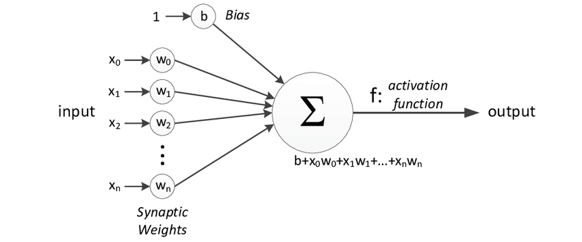
Representation of a neuron, with mathematical symbols showing inputs and outputs

Features of a Neuron

Each neuron has four key characteristics. Let’s discuss each of them.

Input

The features fed into the model during the learning process are referred to as the input. For instance, in the case of object detection, the input may be an array of pixel values from an image.

Weights

Weights serve to emphasize the “features” that have a greater impact on the learning process. The more a feature appears in a successful prediction made by a network, the more weight the neuron(s) that represent that feature are given. Weights are calculated by applying scalar multiplication to the input value and the weight matrix. For instance, a negative word would have more influence on the outcome of a sentiment analysis model tasked with identifying negative words than a pair of neutral words.

Activation Function

The main purpose of an activation function is to transform the summed weighted input from a node into an output value that is passed on to the next hidden layer or used as the final output.
Activation functions determine whether or not a neuron should be activated based on its input to the network. These functions use mathematical operations to decide if the input is important for prediction. If an input is deemed important, the function “activates'' the neuron.

Most activation functions are non-linear. This allows neural networks to "learn" features about a dataset (i.e. how different pixels make up a feature in an image). Without non-linear activation functions, neural networks would only be able to learn linear and affine functions. Why is this an issue? It is an issue because the linear and affine functions cannot capture the complex and non-linear patterns that often exist in real-world data.

Bias

Bias is a term used to refer to the parameters of a neuron that are added to the weighted sum of inputs before passing through the activation function. Bias is typically represented as a scalar value and is learned during the training process of the neural network, along with the weights.

The bias term can change the output of a neuron by shifting the activation function to the left or right, which can change the range of output values and the number of neurons that fire. This can have a significant impact on the overall behavior of the network.

The General Structure of a Neural Network

Neural networks vastly differ. Each day, people around the world in business and academia are experimenting with new configurations for neural networks that solve a given problem better than previous versions. But, generally, there are a few features of a neural network that are consistent across networks.

The following image shows the general structure of a neural network, with an input layer, hidden layers, and output layers:

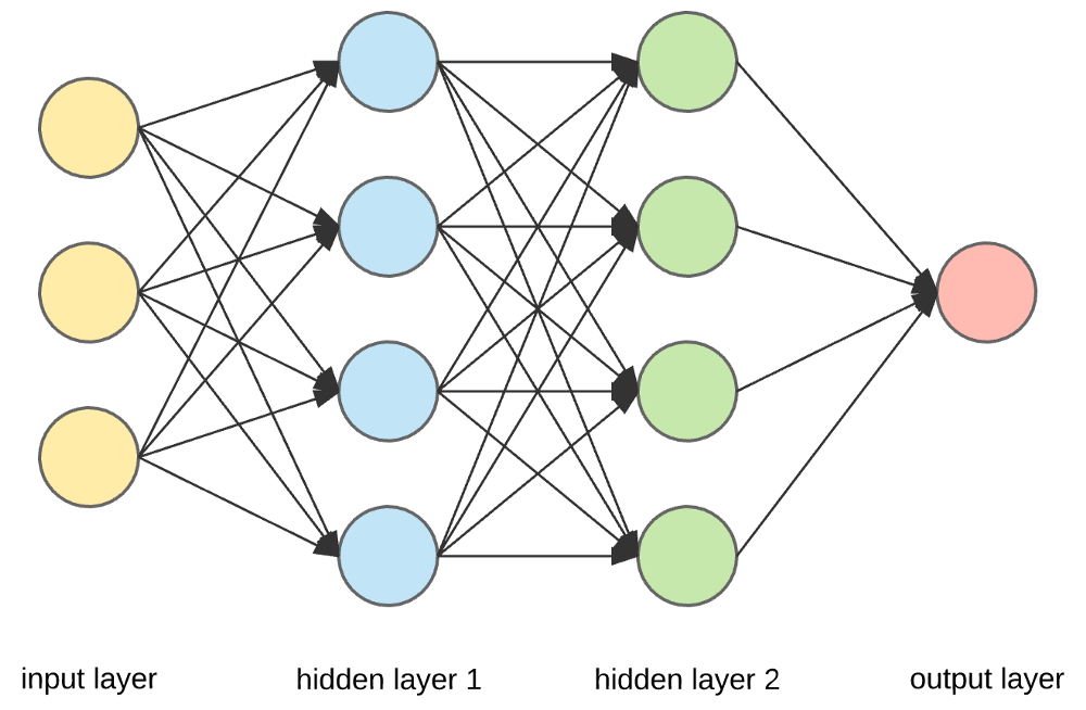
Let’s talk about each of these components.

Input Layer

The input layer of a neural network receives data. This data will have been processed from sources like images or tabular information and reduced into a structure that the network understands. This layer is the only one that is visible in the complete neural network architecture. The input layer passes on the raw data without performing any computation.

Hidden Layer

Hidden layers (pictured in the image above) are the backbone of deep learning. They are the intermediate layers that perform computations and extract features from data. There may be multiple interconnected hidden layers, each responsible for identifying different features in the data. For instance, in image processing, early hidden layers detect high-level features such as edges, shapes, or boundaries while later layers carry out more complex tasks like recognizing complete objects like cars, buildings, or people.

Output Layer

The output layer receives input from the preceding hidden layers and generates a final prediction based on the model's learned information. In classification/regression models, the output layer usually has a single node. But, the number can vary depending on the specific type of problem being solved and how the model was constructed.

Neural Networks Architectures

One of the key factors in the success of neural networks is the architecture of the network, which determines the way in which the network processes and interprets information.

In this section, we will discuss some of the most popular neural network architectures and their applications, including:

1. Perceptrons;
2. Feedforward neural networks;
3. Residual networks (ResNet);
4. LTSM networks;
5. Convolutional neural networks and;
6. Recurrent neural networks.

Understanding the different architectures and their strengths and limitations is crucial for selecting the appropriate network for a given task, achieving optimal performance, and to help you intuitively understand how we got to the current neural networks.

The Perceptron

A perceptron is the most basic neural network architecture. Perceptrons receive multiple inputs, apply mathematical operations on them, and generate an output.

The perceptron accepts a vector of real-value inputs, performs a linear combination of each input with its corresponding weight, sums the weighted inputs, and passes the result through an activation function. Perceptron units can be combined to create more complex Artificial Neural Network architectures.

Feed-Forward Networks

A perceptron models the behavior of a single neuron. When multiple perceptrons are arranged in a sequence and organized into layers, it forms a multi-layer neural network.

In this architecture, information flows in a forward direction, from left to right, starting from the input layer, passing through multiple hidden layers, and finally reaching the output layer. This type of network is known as a feed-forward network, as information does not loop back between hidden layers. The later layers don't provide feedback to the previous ones; learning is one-way. The learning process remains the same as the perceptron.

Residual Networks (ResNet)

Now that you know a bit about feed-forward networks, you may be wondering: how do you determine the number of layers in a neural network architecture?

A common misconception is that the more hidden layers used in a network, the better the learning process. However, this isn't always the case. Neural networks with many layers can be difficult to train because of issues including vanishing and exploding gradients.

One approach to addressing these issues is to use Residual Networks (ResNets). Unlike traditional feed-forward networks, ResNets provide an alternate path for data flow that makes training faster and easier.

ResNets are architected based on the theory that a deep network can be constructed from a shallower network by copying weights from the shallower network using identity mapping. The data from earlier layers is "fast-forwarded" and carried forward in the network through what are called skip connections. These connections were first introduced in ResNets to help solve the vanishing gradient problem.

Recurrent Neural Networks (RNNs)

Traditional deep learning architecture has a fixed input size, which can be a limitation in situations where the input size is not fixed. Additionally, these models make decisions based only on the current input, without considering previous inputs.

Recurrent Neural Networks (RNNs) are well-suited for handling sequences of data as input. They excel in NLP tasks such as sentiment analysis and spam filters, as well as time series problems such as sales forecasting and stock market prediction. RNNs have the ability to "remember" previous inputs and use that information to inform future predictions.

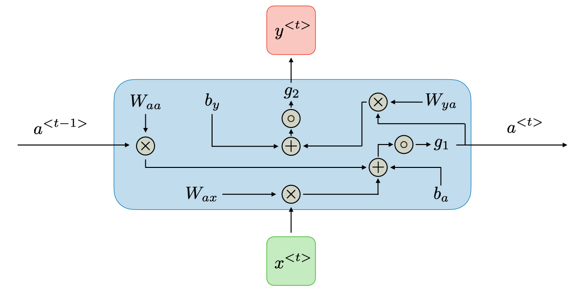
In RNN, sequential data is fed as input. The network has an internal hidden state that gets updated with every new input sequence. This internal hidden state is fed back to the model and it produces an output at each timestamp. At each timestamp, the network receives a new input sequence and updates this internal hidden state based on both the new input and its current hidden state. This updated hidden state is then used to produce an output, which can be a prediction, a classification, or some other kind of decision.

The timestamp refers to the order in which the input sequences are presented to the network. In some applications, such as natural language processing, the timestamp can correspond to the position of a word in a sentence. In other applications, such as time series forecasting, the timestamp can correspond to a point in time.

The internal hidden state is fed back to the model at each timestamp which means the hidden state of previous timestep is passed to the current timestep to make prediction or decision. This allows the network to maintain a "memory" of past inputs and use that information to inform its current output.

The Long Short Term Memory Network (LSTM)

In traditional RNNs, each prediction is based solely on the previous timestamp and it has a limited short-term memory. It doesn't consider information from farther back in time. To improve this, we can expand the recurrent neural network structure by incorporating the concept of “memory”.

We can accomplish this by adding components called gates to the network structure. These gates allow the network to remember information from previous timestamps, enabling it to have a longer-term memory.

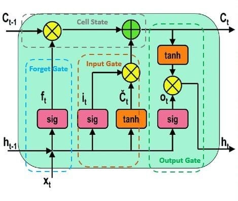
• Cell state (C_t): The cell state, represented as c_t, is related to the long-term memory of the network.
• Forget Gate: The forget gate erases information in the cell state that is no longer useful. It takes in two inputs, the current timestamp input (x_t) and the previous cell state (h_t-1), which are multiplied by their corresponding weight matrices, and then bias is added. The output is passed through an activation function that produces a binary value, which determines if the information is kept or discarded.
• Input gate: The input gate selects which new information should be added to the cell state. It operates similarly to the forget gate, utilizing the current timestamp input and the previous cell state, but with the distinction of utilizing a distinct set of weights for multiplication.
• Output gate: The purpose of the output gate is to identify relevant information from the current cell state and to present it as an output.

Convolutional Neural Networks (CNNs)

Convolutional Neural Networks (CNNs) are a type of feed-forward neural networks that are commonly used for tasks such as image analysis, natural language processing, and other challenging image classification problems.

CNNs consist of hidden layers, known as convolutional layers, that form the foundation of these networks. In image data, features refer to small details such as edges, borders, shapes, textures, objects, circles, etc.

The convolutional layers of a CNN utilize filters to detect these patterns in the image data, with the lower layers focusing on simpler features, and the deeper layers being able to detect more complex features and objects. For example, in later layers, filters may detect specific objects such as eyes or ears, and eventually even animals such as cats and dogs.

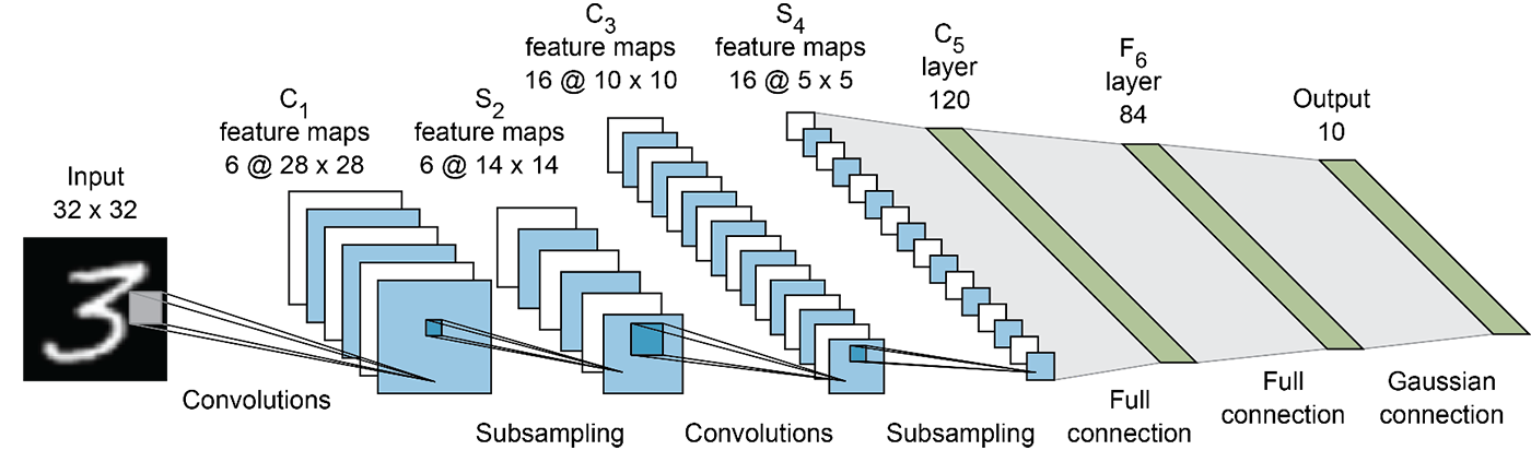
When adding a convolutional layer to a network, the number of filters needs to be specified. A filter can be conceptualized as a small matrix, where the number of rows and columns is chosen. The values in this feature matrix are initialized with random numbers. When the convolutional layer receives pixel values of input data, the filter convolves over each patch of the input matrix. The output from the convolutional layer is usually passed through a ReLU activation function, which brings non-linearity to the model by replacing all negative values with zero.

Pooling is a crucial step in CNNs as it reduces computation and makes the model more robust to distortions and variations. A fully connected dense neural network would then use a flattened feature matrix and make predictions based on the specific use case.

Generative Adversarial Network (GAN)

Generative modeling is a subcategory of unsupervised learning, in which new or synthetic data is produced based on the patterns discovered from a set of input data. Generative Adversarial Networks (GANs) are a type of generative model that can generate entirely new synthetic data by learning patterns in the input data. GANs are a popular and active area of AI research.

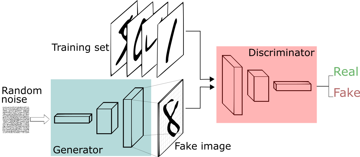
GANs consist of two parts: a generator and a discriminator, that work in a competitive manner. The generator is responsible for creating synthetic data based on the features it learned during the training phase. It takes random data as input and returns a generated image after performing certain transformations. The discriminator acts as a critic and has a general understanding of the problem domain as well as the ability to recognize generated images.

The generator creates images and the discriminator classifies them as either fake or genuine. The discriminator returns a probabilistic prediction in the range of 0 to 1 where 1 represents an authentic image and 0 a fake image. The generator continues to produce samples and the discriminator attempts to distinguish between samples from the training data and samples produced by the generator. The generator receives feedback from the discriminator to improve its performance.

When the discriminator is successful in distinguishing real from fake examples, its parameters do not need to be changed. The generator is penalized when it fails to generate images that can fool the discriminator. However, if it succeeds in making the discriminator categorize the generated image as real, it indicates that the training of the generator is progressing well. The ultimate aim for the generator is to fool the discriminator, while the discriminator's goal is to improve its accuracy.

GANs are used in various applications such as predicting the next frame in a video, text-to-image generation, image-to-image translation, image denoising and more.

Transformers

Training RNNs and LSTMs can be slow and inefficient, especially with large sequenced data and the problem of vanishing gradients. One of the issues is that data needs to be fed in sequentially, which does not take full advantage of GPUs.

To address this issue, Transformers were introduced, which employ an encoder-decoder structure and allow input data to be passed in parallel. Unlike RNNs where input is passed one word at a time, with Transformers there is no concept of timestamps for input, the entire sentence is fed in together and embeddings for all words are produced simultaneously.

For example, in the case of English-French translation, Transformers allow to process the entire input sentence at once, and not one word at a time as in RNNs.

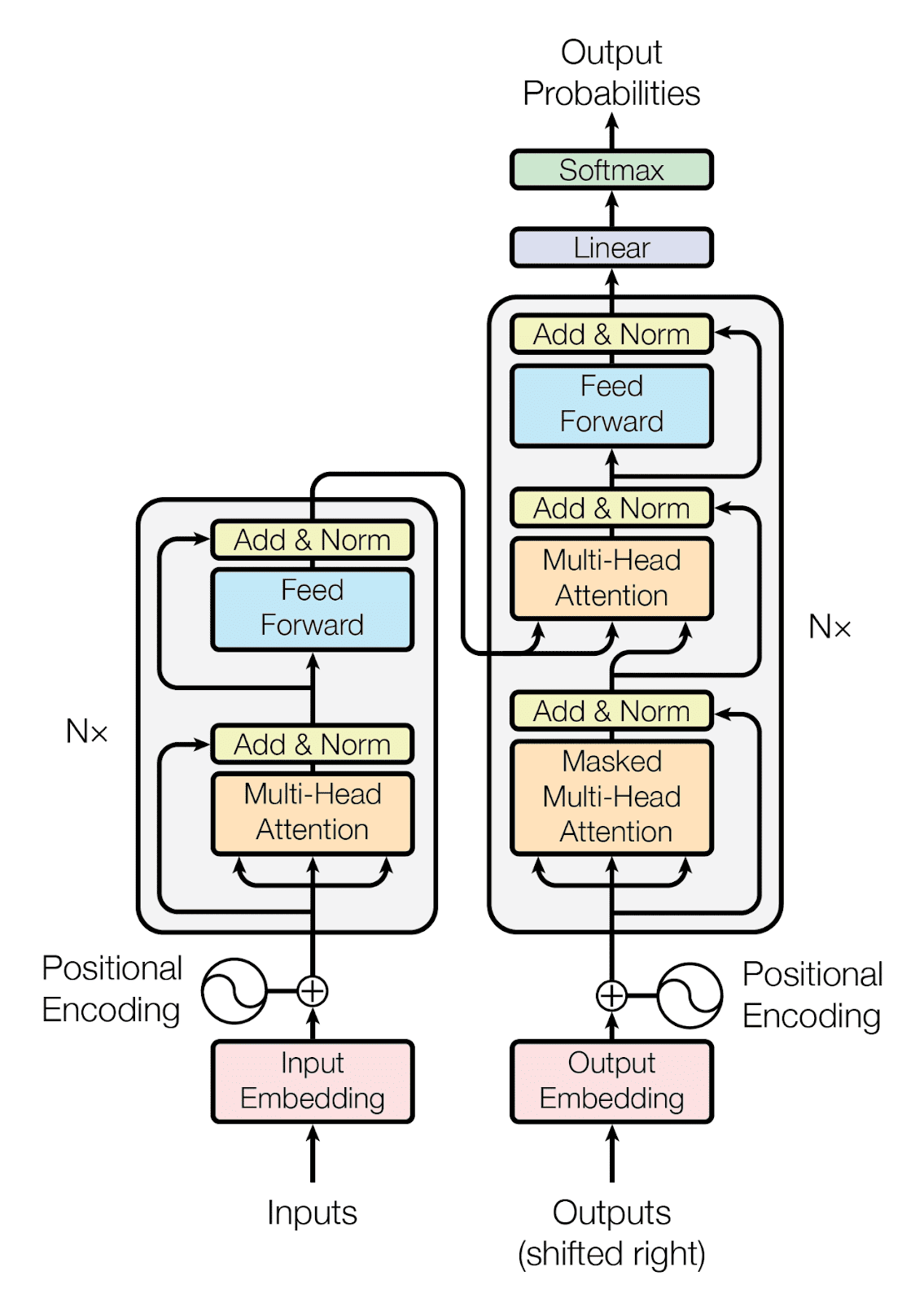
Computers process numbers and vectors, not words. To represent words, they use a technique called word embedding which maps each word to a point in a vector space called the embedding space. A pre-trained embedding space is used to map a word to a vector. However, the same word in different contexts can have different meanings.

Embeddings capture the context of a word based on its position within a sentence. By combining Input Embeddings with Positional Encoding, the resulting embeddings contain context information. This is passed to an encoder block that includes a multi-head attention layer and a feed-forward layer. The attention layer is used to decide which parts of the input sentence are important for the model to focus on. During training, the decoder is fed with corresponding French sentence embeddings which consists of three main components.

The self-attention mechanism in transformer networks generates attention vectors for each word in a sentence, indicating the relevance of each word to all other words in the same sentence. These attention vectors and the encoder's vectors are then processed by the "encoder-decoder attention block," which assesses the relationship between each word vector.

This block is responsible for the mapping from English to French. A significant change in architecture was introduced by replacing RNNs with Transformers. Unlike RNNs, Transformers use parallel computing and have a self-attention mechanism that preserves important information, eliminating the problems of sequential data processing and information loss found in RNNs.

GPT

GPT is a language model that uses generative training and does not require labeled data for its training. It predicts the probability of the sequence of words in a language. There are three version of if so far: GPT-1, GPT-2 and GPT-3.

The GPT-1 model goes through a two-phase training process, beginning with unsupervised pre-training using a large corpus of unlabeled data, using the language model objective function, followed by supervised fine-tuning of the model on a specific task with task-specific data. The GPT-1 model is based on the transformer decoder architecture.

The main focus of GPT-2 is on generating text, it utilizes an autoregressive approach and trains on input sequences with the objective of predicting the next token at each point in the sequence. The model is built using transformer blocks, with a focus on attention mechanism and has less dimensional parameters as compared to BERT, however it contains more transformer blocks (48 blocks) and can process longer sequences.

The architecture of GPT3 is similar to GPT2, but it has a higher number of transformer blocks(96 blocks) and it is trained on a larger dataset. Additionally, the sequence length of the input sentences in GPT3 is double the size of GPT2, resulting in it being the largest neural network architecture with the most parameters.

Key Takeaways On Neural Networks

Each type of neural network architecture has its own strengths and limitations.

Feed-forward neural networks are widely used for solving simple structured data problems like classification and regression.

Recurrent neural networks are more effective in handling sequential data such as text, audio and video.

Recent studies have shown that Transformer networks, which use attention mechanisms, have surpassed RNNs in many areas, and represent the foundation of many of today's state-of-the-art models.