How to Download and Run SAM 3 Weights

Curious how to download SAM 3 weights? Segment Anything 3 (SAM 3) is Meta's latest foundation model for image and video segmentation, released in November 2025. SAM 3 can detect, segment, and track objects using text prompts, point clicks, bounding boxes, image exemplars, or any combination of these.

In this tutorial, you will learn the easiest way to run run SAM 3 on your own machine: the Roboflow inference Python package.

Benefits of Using SAM 3 Through Roboflow

Running SAM 3 from Meta's raw weights requires requesting access to the HuggingFace checkpoints, authenticating, installing the right PyTorch build for your hardware, managing CUDA driver compatibility, and handling platform-specific issues.

Roboflow inference removes all of that friction:

• Zero configuration: The package detects your hardware and configures everything automatically. The right execution providers are selected, model weights are downloaded and cached, and the runtime is optimized for your device. This works the same way on a Windows laptop, a MacBook with Apple Silicon, a Linux workstation, an NVIDIA Jetson, a Raspberry Pi, or a cloud VM. No CUDA toolkits to install, no ONNX runtime to configure, no drivers to patch.
• Works on your hardware as-is: You do not need to match CUDA versions, install specific PyTorch builds, or troubleshoot device-specific driver issues. Whether you are on a consumer laptop or an edge device, the package is ready to go without any customization. See the full list of supported platforms.
• Automatic updates: When new SAM 3 improvements or optimizations are released, the package handles those updates for you. You do not need to track upstream changes in Meta's repository, rebuild environments, or re-export weights.
• Simple API: Initialize the model with one line, pass in an image and text prompts, and get back segmentation masks with confidence scores. See the full SAM 3 API reference.
• Multiple output formats: Polygon, RLE (run-length encoding), and JSON output formats are supported out of the box, so you can choose the format that fits your downstream use case without writing conversion code.
• Text and visual prompts in one package: The package supports both SAM 3's new text-based concept segmentation and the interactive point-and-box segmentation from SAM 2, through a unified API.
• Integration with the Roboflow ecosystem: The same SAM 3 model works with Autodistill for auto-labeling datasets, with the supervision library for visualization, and with the broader Roboflow platform for training smaller models on SAM 3-labeled data.

Using SAM 3 with the Roboflow Inference Package

The Roboflow inference package lets you import SAM 3 Inference directly into your Python script and run the model locally. Running SAM 3 with Inference therefore means you don’t need to do any manual configuration. You won’t have to install PyTorch manually or worry about driver versions. The same commands will work on your laptop, desktop workstation, edge devices or cloud server. In the sections below you will see how simple it is.

Prerequisites

You will need a Roboflow API key. Sign up for a free account and find your key on your Settings page.

Installation

Install the package with SAM 3 support:

uv pip install inference-gpu[sam3]

The [sam3] extra pulls in the specific dependencies SAM 3 needs. When you first run the model, the weights are downloaded automatically and cached locally. Subsequent runs start immediately.

Example 1: Text-Based Concept Segmentation

The defining feature of SAM 3 is its ability to segment objects based on text prompts. You type a short noun phrase, and the model finds and segments every matching instance in the image. This is what Meta calls Promptable Concept Segmentation (PCS). Try the following code example:

from inference.models.sam3 import SegmentAnything3
from inference.core.entities.requests.sam3 import Sam3Prompt

# Initialize the model
# The model will automatically download weights if not present
model = SegmentAnything3(model_id="sam3/sam3_final",   api_key="<ROBOFLOW_API_KEY>")

# Define your image (can be a path, URL, or numpy array)
image_path = "dog-and-cat.jpg"

# Define text prompts
prompts = [
    Sam3Prompt(type="text", text="dog"),
    Sam3Prompt(type="text", text="cat")
]

# Run inference
response = model.segment_image(
    image=image_path,
    prompts=prompts,
    output_prob_thresh=0.5,
    format="polygon" # or "rle", "json"
)

# Process results
for prompt_result in response.prompt_results:
    print(f"Prompt: {prompt_result.echo.text}")
    for prediction in prompt_result.predictions:
        print(f"  Confidence: {prediction.confidence}")
        print(f"  Mask: {prediction.masks}")

The format parameter controls how masks are returned. Use "polygon" for drawing contours, "rle" for compact storage, or "json" for a general-purpose structured response. You can pass any short noun phrase as a prompt. SAM 3 handles a much wider vocabulary than traditional fixed-class models.

Since in the above example, we used format="polygon", each prediction mask is a polygon. The segment_image(..., format="polygon") returns masks in polygon form like shown below:

Prompt: dog
  Confidence: 0.828125
  Mask: [[[229, 559], [229, 560]], [[760, 178], ...
Prompt: cat
  Confidence: 0.8984375
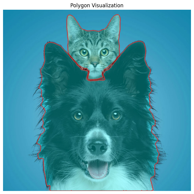
  Mask: [[[638, 29], [637, 30], [635, 30], ...

We can use this information to draw polygon on the original image with OpenCV. The following code visualizes the polygon by converting it to a NumPy array and drawing it with cv.polylines(...).

import cv2 as cv
import numpy as np
import matplotlib.pyplot as plt

# Load original image
img = cv.imread("dog-and-cat.jpg")
img_rgb = cv.cvtColor(img, cv.COLOR_BGR2RGB)

# Make a copy for drawing
overlay = img_rgb.copy()
output = img_rgb.copy()

for prompt_result in response.prompt_results:
    print(f"Prompt: {prompt_result.echo.text}")

    for prediction in prompt_result.predictions:
        print(f"  Confidence: {prediction.confidence}")

        # prediction.masks can contain one or more polygons
        for mask in prediction.masks:
            polygon = np.array(mask, dtype=np.int32)

            # Fill polygon on overlay
            cv.fillPoly(overlay, [polygon], color=(0, 255, 255))

            # Draw polygon border on output
            cv.polylines(output, [polygon], isClosed=True, color=(255, 0, 0), thickness=3)

# Blend overlay with original image for transparent fill
blended = cv.addWeighted(overlay, 0.35, output, 0.65, 0)

plt.figure(figsize=(8, 8))
plt.imshow(blended)
plt.axis("off")
plt.title("Polygon Visualization")
plt.show()

You will see output similar to following:

You can visualize your SAM 3 result nicely with Roboflow Supervision.

The key detail is that Supervision’s segmentation-style annotators such as MaskAnnotator, PolygonAnnotator, and HaloAnnotator use sv.Detections.mask. BackgroundOverlayAnnotator also uses masks when they are present.

Since your SAM 3 response is already returning polygons, the easiest flow is:

1. load the image
2. convert each polygon into a binary mask
3. build an sv.Detections object
4. use Supervision annotators on that object.

Here is a complete working example.

import cv2
import numpy as np
import matplotlib.pyplot as plt
import supervision as sv

# 1. Load original image
image_bgr = cv2.imread("dog-and-cat.jpg")
image_rgb = cv2.cvtColor(image_bgr, cv2.COLOR_BGR2RGB)
h, w = image_rgb.shape[:2]

# 2. Convert SAM3 polygons to Supervision detections
masks = []
xyxy = []
confidences = []
class_ids = []
labels = []

prompt_to_class = {}
next_class_id = 0

for prompt_result in response.prompt_results:
    prompt_text = prompt_result.echo.text

    if prompt_text not in prompt_to_class:
        prompt_to_class[prompt_text] = next_class_id
        next_class_id += 1

    class_id = prompt_to_class[prompt_text]

    for prediction in prompt_result.predictions:
        confidence = float(prediction.confidence)

        for polygon in prediction.masks:
            polygon = np.array(polygon, dtype=np.int32)

            # Skip bad polygons
            if polygon.ndim != 2 or polygon.shape[0] < 3:
                continue

            # Create binary mask
            mask = np.zeros((h, w), dtype=np.uint8)
            cv2.fillPoly(mask, [polygon], 1)

            # Compute bounding box from polygon
            x_min = polygon[:, 0].min()
            y_min = polygon[:, 1].min()
            x_max = polygon[:, 0].max()
            y_max = polygon[:, 1].max()

            masks.append(mask.astype(bool))
            xyxy.append([x_min, y_min, x_max, y_max])
            confidences.append(confidence)
            class_ids.append(class_id)
            labels.append(f"{prompt_text} {confidence:.2f}")

# Build Supervision detections
detections = sv.Detections(
    xyxy=np.array(xyxy, dtype=np.float32),
    mask=np.array(masks, dtype=bool),
    confidence=np.array(confidences, dtype=np.float32),
    class_id=np.array(class_ids, dtype=int),
    data={"labels": np.array(labels, dtype=object)}
)

print(detections)

Filled mask visualization

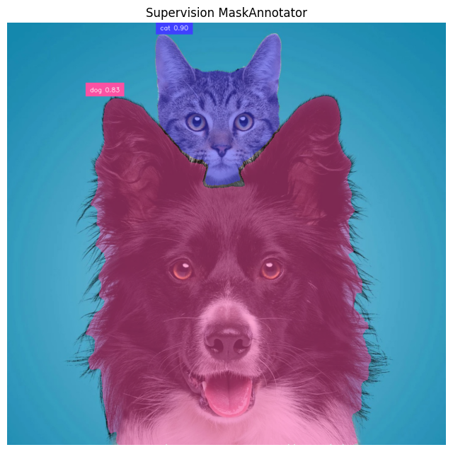
MaskAnnotator is the best choice when you want the segmented object area filled. Supervision provides sv.Detections.mask annotator. Here's the example how to use it:

mask_annotator = sv.MaskAnnotator()
label_annotator = sv.LabelAnnotator(text_position=sv.Position.TOP_LEFT)

annotated = image_rgb.copy()
annotated = mask_annotator.annotate(scene=annotated, detections=detections)
annotated = label_annotator.annotate(
    scene=annotated,
    detections=detections,
    labels=labels
)

plt.figure(figsize=(8, 8))
plt.imshow(annotated)
plt.axis("off")
plt.title("Supervision MaskAnnotator")
plt.show()

Following will be the output of the above code.

Polygon outline visualization

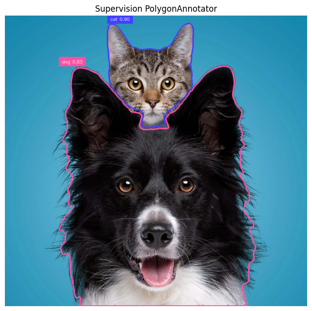
PolygonAnnotator draws the segmentation boundary from masks. The PolygonAnnotator also uses sv.Detections.mask. Here's the code:

polygon_annotator = sv.PolygonAnnotator(thickness=3)
label_annotator = sv.LabelAnnotator(text_position=sv.Position.TOP_LEFT)

annotated = image_rgb.copy()
annotated = polygon_annotator.annotate(scene=annotated, detections=detections)
annotated = label_annotator.annotate(
    scene=annotated,
    detections=detections,
    labels=labels
)

plt.figure(figsize=(8, 8))
plt.imshow(annotated)
plt.axis("off")
plt.title("Supervision PolygonAnnotator")
plt.show()

You will see output similar to following.

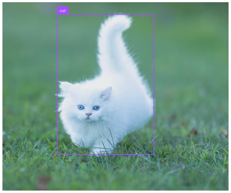
Bounding box visualization

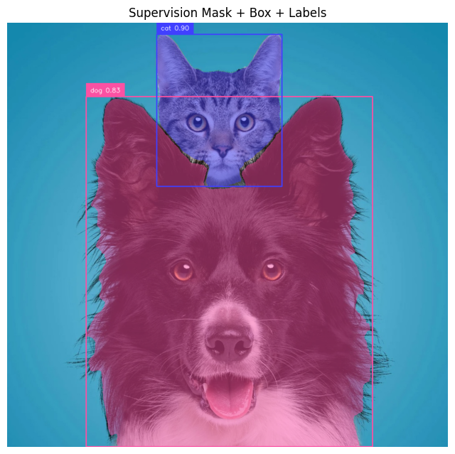
Supervision’s Detections object is the common format used with annotators, and bounding-box annotators can be layered with segmentation annotators. Here's the code:

mask_annotator = sv.MaskAnnotator()
box_annotator = sv.BoxAnnotator()
label_annotator = sv.LabelAnnotator(text_position=sv.Position.TOP_LEFT)

annotated = image_rgb.copy()
annotated = mask_annotator.annotate(scene=annotated, detections=detections)
annotated = box_annotator.annotate(scene=annotated, detections=detections)
annotated = label_annotator.annotate(
    scene=annotated,
    detections=detections,
    labels=labels
)

plt.figure(figsize=(8, 8))
plt.imshow(annotated)
plt.axis("off")
plt.title("Supervision Mask + Box + Labels")
plt.show()

You will see output similar to following with the above code.

Example 2: Interactive Segmentation (Points)

SAM 3 also supports the interactive segmentation workflow from SAM 2. You click on an object (or draw a bounding box) and the model generates a segmentation mask for that specific instance. This is handled by the Sam3ForInteractiveImageSegmentation class and is ideal for human-in-the-loop annotation tools. Follow the example below to achieve this.

First, download the SAM 3 weights.

import numpy as np
import matplotlib.pyplot as plt
import supervision as sv

from inference.models.sam3 import Sam3ForInteractiveImageSegmentation

image_path = "cat.jpg"
image_bgr = cv2.imread(image_path)
image_rgb = cv2.cvtColor(image_bgr, cv2.COLOR_BGR2RGB)

# Load interactive SAM 3 model
model = Sam3ForInteractiveImageSegmentation(
    model_id="sam3/sam3_final",
    api_key="ROBOFLOW_API_KEY"   # put your API key
)

Embed image and specify interactive prompts (points).

embedding, img_shape, image_id = model.embed_image(image=image_path)


# Interactive prompts
# positive=True  -> include
# positive=False -> exclude
points = [
    {"x": 394, "y": 328, "positive": True}, 
]

masks, scores, logits = model.segment_image(
    image=image_path,
    image_id=image_id,
    prompts={"points": points}
)

print("scores:", scores)

Convert the masks returned by the interactive SAM3 point prompt into Supervision detections so they can be visualized with mask, polygon, box, and label annotators.

masks_np = np.array(masks)

if masks_np.ndim == 2:
    masks_np = masks_np[None, :, :]

masks_bool = masks_np > 0

xyxy = []
for mask in masks_bool:
    ys, xs = np.where(mask)
    if len(xs) == 0 or len(ys) == 0:
        xyxy.append([0, 0, 0, 0])
    else:
        xyxy.append([xs.min(), ys.min(), xs.max(), ys.max()])

detections = sv.Detections(
    xyxy=np.array(xyxy, dtype=np.float32),
    mask=masks_bool,
    confidence=np.array(scores[:len(masks_bool)], dtype=np.float32),
)

labels = [f"mask {score:.2f}" for score in detections.confidence]

Use Supervision to draw the interactive SAM3 masks, polygon outlines on the image and then displays the final annotated result.

mask_annotator = sv.MaskAnnotator(color_lookup=sv.ColorLookup.INDEX)
polygon_annotator = sv.PolygonAnnotator(thickness=2, color_lookup=sv.ColorLookup.INDEX)

annotated = image_rgb.copy()
annotated = mask_annotator.annotate(scene=annotated, detections=detections)
annotated = polygon_annotator.annotate(scene=annotated, detections=detections)

plt.figure(figsize=(8, 8))
plt.imshow(annotated)
plt.axis("off")
plt.title("Interactive SAM 3")
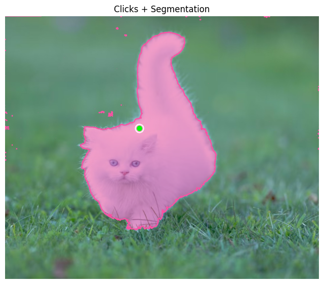
plt.show()

Now, draw clicked points (green for positive, red for negative) on top of the segmented image so you can visually see where you clicked along with the segmentation result. The output will be similar to folowing.

Example 3: Auto-Labeling with Autodistill + SAM 3

SAM 3 is powerful but compute-intensive. In many production scenarios, you need a smaller, faster model that can run in real time on edge hardware. The typical workflow is to use SAM 3 to automatically label a dataset, then train a smaller supervised model (like RF-DETR) on those labels.

Autodistill automates this process. You define an ontology that maps text prompts to class names, point Autodistill at a folder of unlabeled images, and it generates labeled annotations using SAM 3 as the base model.

Install with pip install autodistill-sam3 (GPU required) and set export ROBOFLOW_API_KEY=YOUR_KEY.

pip install -U inference autodistill autodistill-sam3

Set the API key.

import os
os.environ["ROBOFLOW_API_KEY"] = "ROBOFLOW_API_KEY"

Download the model weight.

from autodistill_sam3 import SegmentAnything3
from autodistill.detection import CaptionOntology

base_model = SegmentAnything3(
    ontology=CaptionOntology({
        "cat": "cat",
        "dog": "dog"
    })
)

print("base model initialized")

Load and annotate image.

from autodistill.helpers import load_image
import supervision as sv

detections = base_model.predict("dog-and-cat.jpg")
image = load_image("dog-and-cat.jpg", return_format="cv2")

mask_annotator = sv.MaskAnnotator(color_lookup=sv.ColorLookup.INDEX)
label_annotator = sv.LabelAnnotator(
    text_position=sv.Position.CENTER,
    color_lookup=sv.ColorLookup.INDEX
)

annotated_frame = mask_annotator.annotate(scene=image.copy(), detections=detections)
annotated_frame = label_annotator.annotate(
    scene=annotated_frame,
    detections=detections,
    labels=[base_model.ontology.classes()[i] for i in detections.class_id]
)

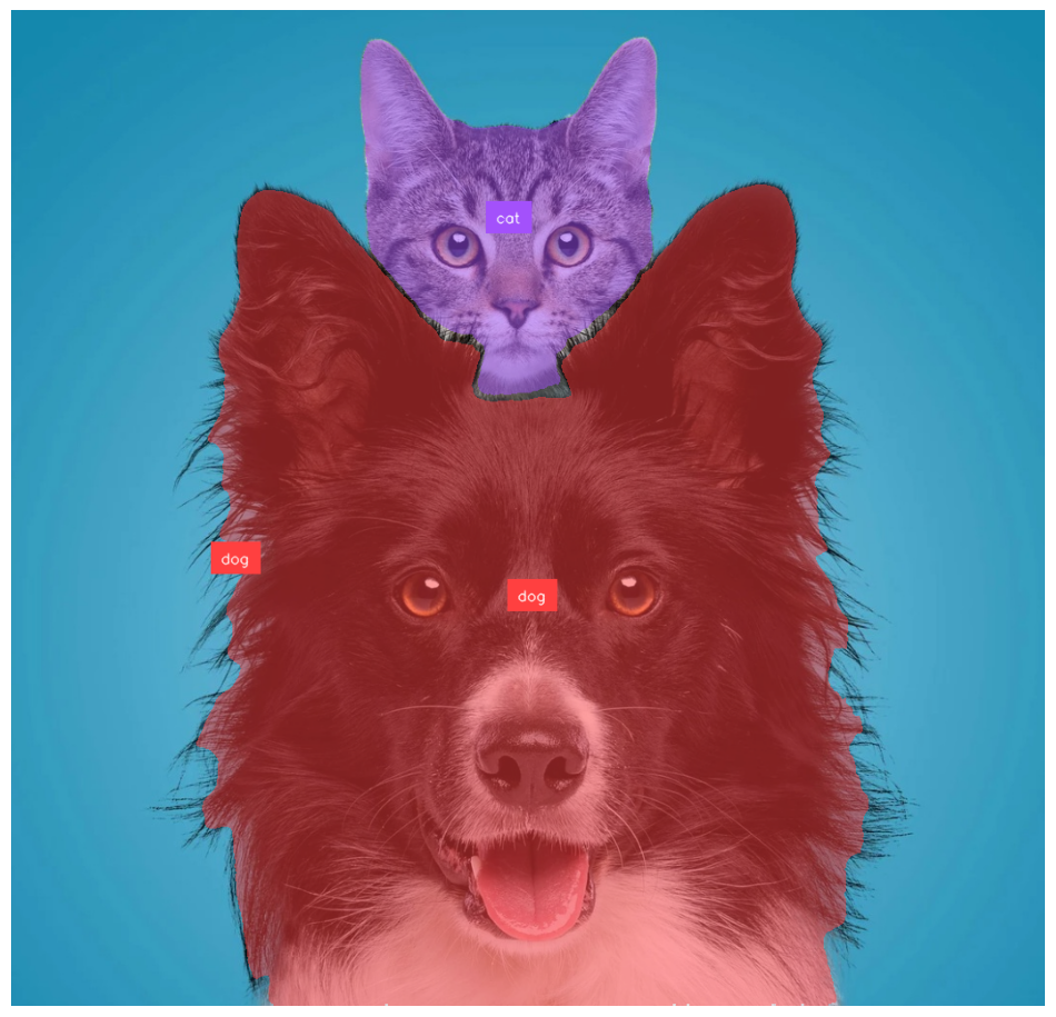
sv.plot_image(annotated_frame)

Running the code will give you output similar to following:

To label an entire folder of images and generate a dataset:

dataset = base_model.label(
    input_folder="/dataset",
    extension=".jpg"
)

print("Labeling complete")
print(dataset)

Using Supervision, you may visualize few training images with following code.

import supervision as sv

dataset = sv.DetectionDataset.from_yolo(
    images_directory_path="/train/images",
    annotations_directory_path="/train/labels",
    data_yaml_path="data.yaml"
)

box_annotator = sv.BoxAnnotator(color_lookup=sv.ColorLookup.CLASS)
label_annotator = sv.LabelAnnotator(color_lookup=sv.ColorLookup.CLASS)

count = 0
for image_name, image, detections in dataset:
    labels = [dataset.classes[i] for i in detections.class_id]

    annotated = image.copy()
    annotated = box_annotator.annotate(scene=annotated, detections=detections)
    annotated = label_annotator.annotate(
        scene=annotated,
        detections=detections,
        labels=labels
    )

    print(image_name)
    sv.plot_image(annotated)

    count += 1
    if count == 5:
        break

It will generate output as following.

The output dataset can be uploaded directly to Roboflow for training a smaller, faster model.

Downloading the SAM 3 Weights

If you prefer to work with the raw model weights directly, Meta has open-sourced the full SAM 3 codebase and checkpoints at github.com/facebookresearch/sam3.

You will need to request access to the checkpoints on the SAM 3 Hugging Face repository and authenticate with your Hugging Face account. Then install with following commands.

git clone https://github.com/facebookresearch/sam3.git
%cd /content/sam3
pip install -q -e .
pip install -q -e ".[notebooks]"

Now login to Hugging Face account.

from huggingface_hub import login
login()

Then use the following code.

import torch
from PIL import Image
from sam3.model_builder import build_sam3_image_model
from sam3.model.sam3_image_processor import Sam3Processor

model = build_sam3_image_model()
processor = Sam3Processor(model)

image = Image.open("cat.jpg")
inference_state = processor.set_image(image)

output = processor.set_text_prompt(state=inference_state, prompt="cat")
masks, boxes, scores = output["masks"], output["boxes"], output["scores"]

When using the raw weights, you are responsible for managing all dependencies, hardware configuration, CUDA setup, and runtime optimization yourself. The repository includes example notebooks for batched inference, video segmentation, interactive segmentation, using SAM 3 as a tool for multimodal LLMs, and running evaluations on the SA-Co benchmark.

SAM 3 Weight Download Conclusion

The Roboflow Inference package gives you the fastest path to running SAM 3 on your own device. Install the package, set your API key, and start segmenting.

Cite this Post

Use the following entry to cite this post in your research:

Timothy M. (Mar 26, 2026). How to Download and Run SAM 3 Weights. Roboflow Blog: https://blog.roboflow.com/download-sam-3-weights/