Edge Detection in Image Processing: An Introduction

This guide explains the concepts behind edge detection (edge models, intensity functions, first and second derivatives), walks through six classical algorithms with runnable OpenCV code (Sobel, Canny, Laplacian, Prewitt, Roberts Cross, and Scharr), shows a crack detection example, and covers when classical edge detection is the right tool versus when a trained model does the job better.

What Is Edge Detection?

Edge detection is an image processing technique for locating the boundaries of objects in an image. Edges appear where pixel intensity changes suddenly, the outline of a part against a conveyor belt, the boundary between a crack and intact concrete. Edge detection algorithms highlight these discontinuities, producing an edge map that later pipeline stages use for object counting, measurement, feature extraction, and segmentation.

The classical algorithms fall into two families. Gradient-based methods (Sobel, Prewitt, Scharr, and the gradient stage of Canny) find edges where the first derivative of intensity peaks. Gaussian-based methods smooth the image first and use second-order derivatives, like the Laplacian, finding edges at zero-crossings. Understanding that split gives each of the six algorithms below a clear place.

Edge Detection Concepts

Let’s talk through a few of the main concepts you need to know to understand edge detection and how it works.

Edge Models

Edge models are theoretical constructs used to describe and understand the different types of edges that can occur in an image. These models help in developing algorithms for edge detection by categorizing the types of intensity changes that signify edges. The basic edge models are Step, Ramp and Roof.  A step edge represents an abrupt change in intensity, where the image intensity transitions from one value to another in a single step. A ramp edge describes a gradual transition in intensity over a certain distance, rather than an abrupt change. A roof edge represents a peak or ridge in the intensity profile, where the intensity increases to a maximum and then decreases.

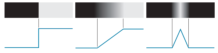
Image Intensity Function

The image intensity function represents the brightness or intensity of each pixel in a grayscale image. In a color image, the intensity function can be extended to include multiple channels (e.g., red, green, blue in RGB images).

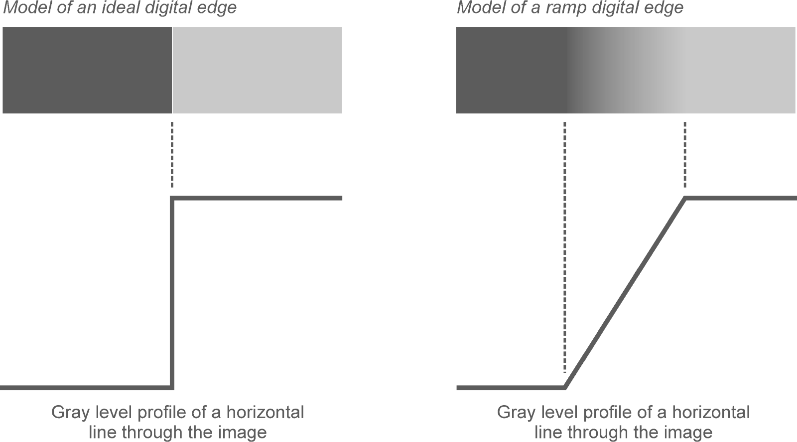
First and Second Derivative

The first derivative of an image measures the rate of change of pixel intensity. It is useful for detecting edges because edges are locations in the image where the intensity changes rapidly. It detects edges by identifying significant changes in intensity. The first derivative can be approximated using gradient operators like the Sobel, Prewitt, or Scharr operators.

The second derivative measures the rate of change of the first derivative. It is useful for detecting edges because zero-crossings (points where the second derivative changes sign) often correspond to edges. It detects edges by identifying zero-crossings in the rate of change of intensity. The second derivative can be approximated using the Laplacian operator. 

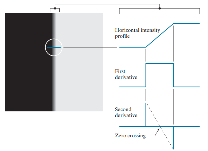
Edge Detection Approaches

There are several approaches to edge detection. Let's talk about the most common approaches one by one.

Sobel Edge Detection

Sobel edge detection is a popular technique used in image processing and computer vision for detecting edges in an image. It is a gradient-based method that uses convolution operations with specific kernels to calculate the gradient magnitude and direction at each pixel in the image. Here's a detailed explanation of Sobel edge detection.

The Sobel operator uses two 3x3 convolution kernels (filters), one for detecting changes in the x-direction (horizontal edges) and one for detecting changes in the y-direction (vertical edges). These kernels are used to compute the gradient of the image intensity at each point, which helps in detecting the edges. Here are the Sobel kernels:

Horizontal Kernel (𝐺𝑥):

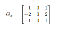
The 𝐺𝑥 kernel emphasizes changes in intensity in the horizontal direction. The positive values (+1 and +2) on the right side will highlight bright areas, while the negative values (-1 and -2) on the left side will highlight dark areas, effectively detecting horizontal edges.

 Vertical Kernel (𝐺𝑦):

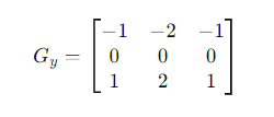
​ The 𝐺𝑦 kernel emphasizes changes in intensity in the vertical direction. Similarly, the positive values (+1 and +2) at the bottom will highlight bright areas, while the negative values (-1 and -2) at the top will highlight dark areas, effectively detecting vertical edges.

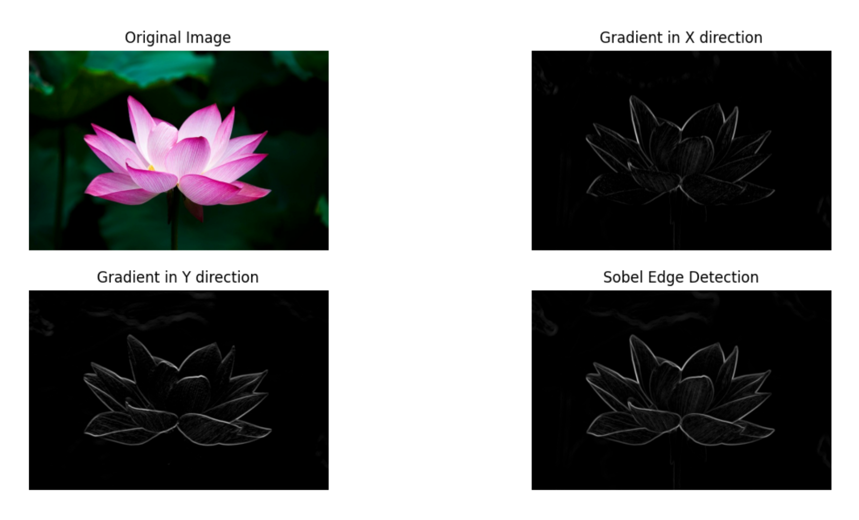
Let's walk through an example of Sobel edge detection using Python and the OpenCV library. Here’s the Step-by-Step Example:

1. Load and Display the Image: First, we need to load a sample image and display it to understand what we're working with.
2. Convert to Grayscale: Convert the image to grayscale as the Sobel operator works on single-channel images.
3. Apply Gaussian Smoothing (Optional): Apply a Gaussian blur to reduce noise and make edge detection more robust.
4. Apply Sobel Operator: Use the Sobel operator to calculate the gradients in the x and y directions.
5. Calculate Gradient Magnitude: Compute the gradient magnitude from the gradients in the x and y directions. A threshold is applied to the gradient magnitude image to classify pixels as edges or non-edges. Pixels with gradient magnitude above the threshold are considered edges.
6. Normalization: The gradient magnitude and individual gradients are normalized to the range 0-255 for better visualization.
7. Display the Resulting Edge Image: Normalize and display the edge-detected image.

import cv2
import numpy as np
import matplotlib.pyplot as plt

# Load the image
image_path = 'flower.jpg'  # Replace with your image path
image = cv2.imread(image_path)

# Convert to grayscale
gray_image = cv2.cvtColor(image, cv2.COLOR_BGR2GRAY)

# Apply Gaussian smoothing (optional)
blurred_image = cv2.GaussianBlur(gray_image, (3, 3), 0)

# Sobel operators
Gx = cv2.Sobel(blurred_image, cv2.CV_64F, 1, 0, ksize=3)
Gy = cv2.Sobel(blurred_image, cv2.CV_64F, 0, 1, ksize=3)

# Gradient magnitude
G = np.sqrt(Gx**2 + Gy**2)

# Normalize to range 0-255
Gx = np.uint8(255 * np.abs(Gx) / np.max(Gx))
Gy = np.uint8(255 * np.abs(Gy) / np.max(Gy))
G = np.uint8(255 * G / np.max(G))

# Display the results
plt.figure(figsize=(15, 10))

# Original image
plt.subplot(2, 2, 1)
plt.imshow(cv2.cvtColor(image, cv2.COLOR_BGR2RGB))
plt.title('Original Image')
plt.axis('off')

# Gradient in X direction
plt.subplot(2, 2, 2)
plt.imshow(Gx, cmap='gray')
plt.title('Gradient in X direction')
plt.axis('off')

# Gradient in Y direction
plt.subplot(2, 2, 3)
plt.imshow(Gy, cmap='gray')
plt.title('Gradient in Y direction')
plt.axis('off')

# Edge-detected image
plt.subplot(2, 2, 4)
plt.imshow(G, cmap='gray')
plt.title('Sobel Edge Detection')
plt.axis('off')

plt.show()

Here, in the following code for sobel operator cv2.CV_64F specifies the desired depth of the output image. Using a higher depth helps in capturing precise gradient values, especially when dealing with small or fine details. For 𝐺𝑥 the values (1, 0) means taking the first derivative in the x-direction and zero derivative in the y-direction. For 𝐺𝑦 the values (0, 1) means taking the first derivative in the y-direction and zero derivative in the x-direction. ksize=3 specifies the size of the extended 3x3 Sobel kernel.

# Sobel operators
Gx = cv2.Sobel(blurred_image, cv2.CV_64F, 1, 0, ksize=3)
Gy = cv2.Sobel(blurred_image, cv2.CV_64F, 0, 1, ksize=3)

The following is the output generated by the code.

Canny Edge Detection

Canny Edge Detection is a multi-stage algorithm to detect a wide range of edges in images. It was developed by John F. Canny in 1986 and is known for its optimal edge detection capabilities. The algorithm follows a series of steps to reduce noise, detect edges, and improve the accuracy of edge detection.

Following are the steps of steps of Canny Edge Detection:

1. Noise Reduction using Gaussian Blurring: The first step in the Canny edge detection algorithm is to smooth the image using a Gaussian filter. This helps in reducing noise and unwanted details in the image. The Gaussian filter is applied to the image to convolve it with a Gaussian kernel. The Gaussian kernel (or Gaussian function) is defined as:

2. Gradient Calculation: 

After noise reduction, the Sobel operator is used to calculate the gradient intensity and direction of the image. This involves calculating the intensity gradients in the x and y directions (𝐺𝑥 and 𝐺𝑦).  The gradient magnitude and direction are then computed using these gradients.

3. Non-Maximum Suppression: To thin out the edges and get rid of spurious responses to edge detection, non-maximum suppression is applied. This step retains only the local maxima in the gradient direction. The idea is to traverse the gradient image and suppress any pixel value that is not considered to be an edge, i.e., any pixel that is not a local maximum along the gradient direction.

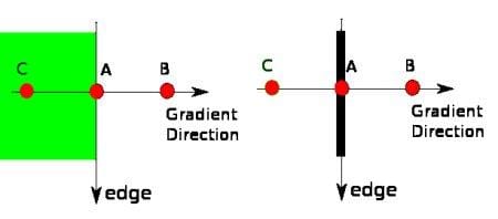
In the above image, point A is located on the edge in the vertical direction. The gradient direction is perpendicular to the edge. Points B and C lie along the gradient direction. Therefore, Point A is compared with Points B and C to determine if it represents a local maximum. If it does, Point A proceeds to the next stage; otherwise, it is suppressed and set to zero.

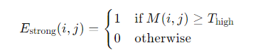
4. Double Thresholding: After non-maximum suppression, the edge pixels are marked using double thresholding. This step classifies the edges into strong, weak, and non-edges based on two thresholds: high and low. Strong edges are those pixels with gradient values above the high threshold, while weak edges are those with gradient values between the low and high thresholds.

Given the gradient magnitude 𝑀 and two thresholds 𝑇_high and 𝑇_low, the classification can be mathematically expressed as:

5. Edge Tracking by Hysteresis: The final step is edge tracking by hysteresis, which involves traversing the image to determine which weak edges are connected to strong edges. Only the weak edges connected to strong edges are retained, as they are considered true edges. This step ensures that noise and small variations are ignored, resulting in cleaner edge detection.

To simplify the process of Canny Edge detection, OpenCV provides cv.Canny() function. Following is the code for Canny Edge detection.

import cv2
import numpy as np
import matplotlib.pyplot as plt

# Load the image
image_path = 'flower.jpg'  # Replace with your image path
image = cv2.imread(image_path, cv2.IMREAD_COLOR)
gray_image = cv2.cvtColor(image, cv2.COLOR_BGR2GRAY)

# Apply Gaussian blur to reduce noise
blurred_image = cv2.GaussianBlur(gray_image, (5, 5), 1.4)

# Apply Canny edge detector
edges = cv2.Canny(blurred_image, 100, 200)

# Display the result
plt.figure(figsize=(10, 5))

# Original image
plt.subplot(1, 2, 1)
plt.imshow(cv2.cvtColor(image, cv2.COLOR_BGR2RGB))
plt.title('Original Image')
plt.axis('off')

# Edge-detected image
plt.subplot(1, 2, 2)
plt.imshow(edges, cmap='gray')
plt.title('Canny Edge Detection')
plt.axis('off')

plt.show()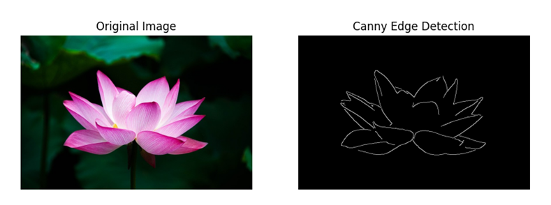

Laplacian Edge Detection

Laplacian Edge Detection is a technique in image processing used to highlight areas of rapid intensity change, which are often associated with edges in an image. Unlike gradient-based methods such as Sobel and Canny, which use directional gradients, Laplacian Edge Detection relies on the second derivative of the image intensity.

Following are the key Concepts of Laplacian Edge Detection:

The Laplacian operator is used to detect edges by calculating the second derivative of the image intensity. Mathematically, the second derivative of an image 𝑓(𝑥, 𝑦) can be represented as:

This can be implemented using convolution with a Laplacian kernel. Common 3x3 kernels for the Laplacian operator include:

cv.Laplacian() is a function provided by the OpenCV library used for performing Laplacian edge detection on images. This function applies the Laplacian operator to the input image to compute the second derivative of the image intensity. Following are the steps for Edge Detection Using Laplacian

1. Convert the Image to Grayscale: Edge detection usually starts with a grayscale image to simplify computations.
2. Apply Gaussian Blur (Optional): Smoothing the image with a Gaussian blur can reduce noise and prevent false edge detection.
3. Apply the Laplacian Operator: Convolve the image with a Laplacian kernel to calculate the second derivative.

import cv2
import numpy as np
import matplotlib.pyplot as plt

# Load the image
image_path = 'flower.jpg'  # Replace with your image path
image = cv2.imread(image_path, cv2.IMREAD_COLOR)
gray_image = cv2.cvtColor(image, cv2.COLOR_BGR2GRAY)

# Optional: Apply Gaussian blur to reduce noise
blurred_image = cv2.GaussianBlur(gray_image, (3, 3), 0)

# Apply the Laplacian operator
laplacian = cv2.Laplacian(blurred_image, cv2.CV_64F)

# Convert the result to 8-bit (0-255) range
laplacian_abs = cv2.convertScaleAbs(laplacian)

# Display the result
plt.figure(figsize=(10, 5))

# Original image
plt.subplot(1, 2, 1)
plt.imshow(cv2.cvtColor(image, cv2.COLOR_BGR2RGB))
plt.title('Original Image')
plt.axis('off')

# Laplacian edge-detected image
plt.subplot(1, 2, 2)
plt.imshow(laplacian_abs, cmap='gray')
plt.title('Laplacian Edge Detection')
plt.axis('off')

plt.show()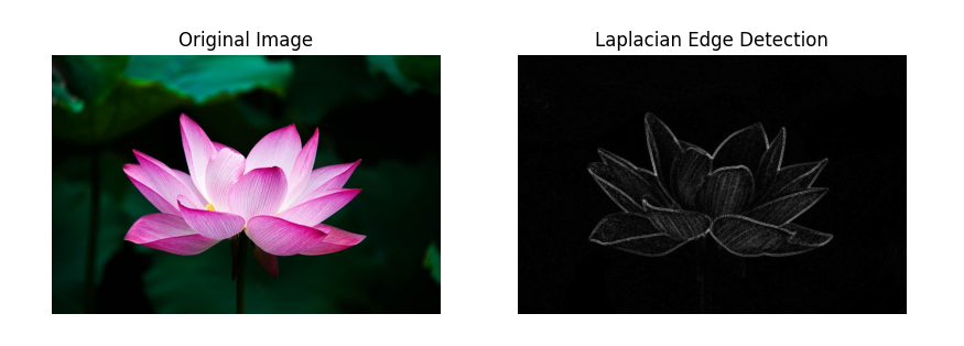

Prewitt Edge Detection

Prewitt edge detection is a technique used for detecting edges in digital images. It works by computing the gradient magnitude of the image intensity using convolution with Prewitt kernels. The gradients are then used to identify significant changes in intensity, which typically correspond to edges.

Prewitt edge detection uses two kernels, one for detecting edges in the horizontal direction and the other for the vertical direction. These kernels are applied to the image using convolution.

Following are the steps in Prewitt Edge Detection

1. Convert the Image to Grayscale: Prewitt edge detection typically operates on grayscale images. If the input image is in color, it needs to be converted to a single channel (grayscale) image.
2. Apply the Horizontal and Vertical Prewitt Kernels: Convolve the image with the horizontal Prewitt kernel (Gx) to detect horizontal edges and with the vertical Prewitt kernel (Gy) to detect vertical edges.
3. Compute Gradient Magnitude: Combine the horizontal and vertical edge maps to compute the gradient magnitude of the image intensity at each pixel. The gradient magnitude represents the strength of the edge at each pixel.
4. Thresholding (Optional): Apply a threshold to the gradient magnitude image to highlight significant edges and suppress noise. Thresholding helps in identifying prominent edges while reducing false detections.

import cv2
import numpy as np
import matplotlib.pyplot as plt

def prewitt_edge_detection(image):
    # Convert the image to grayscale
    gray_image = cv2.cvtColor(image, cv2.COLOR_BGR2GRAY)
    
    # Apply horizontal Prewitt kernel
    kernel_x = np.array([[-1, 0, 1],
                         [-1, 0, 1],
                         [-1, 0, 1]])
    horizontal_edges = cv2.filter2D(gray_image, -1, kernel_x)
    
    # Apply vertical Prewitt kernel
    kernel_y = np.array([[-1, -1, -1],
                         [0, 0, 0],
                         [1, 1, 1]])
    vertical_edges = cv2.filter2D(gray_image, -1, kernel_y)    
    # Ensure both arrays have the same data type
    horizontal_edges = np.float32(horizontal_edges)
    vertical_edges = np.float32(vertical_edges)
    
    # Compute gradient magnitude
    gradient_magnitude = cv2.magnitude(horizontal_edges, vertical_edges)
    
    # Optional: Apply thresholding to highlight edges
    threshold = 50
    _, edges = cv2.threshold(gradient_magnitude, threshold, 255, cv2.THRESH_BINARY)
    
    return edges

# Read the input image
image = cv2.imread('flower.jpg')

# Apply Prewitt edge detection
edges = prewitt_edge_detection(image)

# Plotting both images using subplots
plt.figure(figsize=(10, 5))

# Original Image
plt.subplot(1, 2, 1)
plt.imshow(cv2.cvtColor(image, cv2.COLOR_BGR2RGB))
plt.title('Original Image')
plt.axis('off')

# Detected Edges
plt.subplot(1, 2, 2)
plt.imshow(edges, cmap='gray')
plt.title('Prewitt Edge Detection')
plt.axis('off')

plt.show()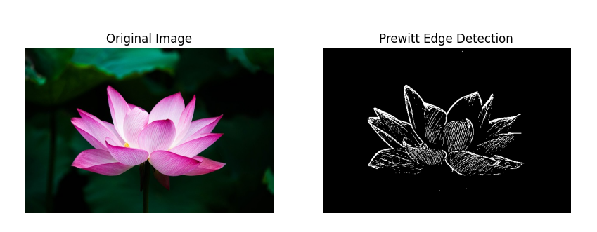

Roberts Cross Edge Detection

Roberts Cross edge detection is a simple technique used for detecting edges in digital images. It works by computing the gradient magnitude of the image intensity using convolution with Roberts Cross kernels. These kernels are small, simple, and efficient for detecting edges, especially when the edges are thin and prominent. Lawrence Roberts first introduced it in 1963 as one of the earliest edge detectors.

Roberts Cross edge detection uses two kernels, one for detecting edges in the horizontal direction and the other for the vertical direction. These kernels are applied to the image using convolution.

Following are the steps in Roberts Cross Edge Detection

1. Convert the Image to Grayscale: Roberts Cross edge detection typically operates on grayscale images. If the input image is in color, it needs to be converted to a single channel (grayscale) image.
2. Apply the Horizontal and Vertical Roberts Cross Kernels: Convolve the image with the horizontal Roberts Cross kernel (Gx) to detect horizontal edges and with the vertical Roberts Cross kernel (Gy) to detect vertical edges.
3. Compute Gradient Magnitude: Combine the horizontal and vertical edge maps to compute the gradient magnitude of the image intensity at each pixel. The gradient magnitude represents the strength of the edge at each pixel.
4. Thresholding (Optional): Apply a threshold to the gradient magnitude image to highlight significant edges and suppress noise. Thresholding helps in identifying prominent edges while reducing false detections.

import cv2
import numpy as np
import matplotlib.pyplot as plt

def roberts_cross_edge_detection(image):
    # Convert the image to grayscale
    gray_image = cv2.cvtColor(image, cv2.COLOR_BGR2GRAY)
    
    # Apply Roberts Cross kernels
    kernel_x = np.array([[1, 0],
                         [0, -1]])
    kernel_y = np.array([[0, 1],
                         [-1, 0]])
                         
    # Convolve the image with the kernels
    horizontal_edges = cv2.filter2D(gray_image, -1, kernel_x)
    vertical_edges = cv2.filter2D(gray_image, -1, kernel_y)
    
    # Ensure both arrays have the same data type
    horizontal_edges = np.float32(horizontal_edges)
    vertical_edges = np.float32(vertical_edges)
    
    # Compute gradient magnitude
    gradient_magnitude = cv2.magnitude(horizontal_edges, vertical_edges)
    
    # Apply thresholding to highlight edges
    threshold = 50
    _, edges = cv2.threshold(gradient_magnitude, threshold, 255, cv2.THRESH_BINARY)
    
    return edges

# Read the input image
image = cv2.imread('flower.jpg')

# Apply Roberts Cross edge detection with thresholding
edges = roberts_cross_edge_detection(image)

# Plotting both images using subplots
plt.figure(figsize=(10, 5))

# Original Image
plt.subplot(1, 2, 1)
plt.imshow(cv2.cvtColor(image, cv2.COLOR_BGR2RGB))
plt.title('Original Image')
plt.axis('off')

# Detected Edges
plt.subplot(1, 2, 2)
plt.imshow(edges, cmap='gray')
plt.title('Roberts Cross Edge Detection with Thresholding')
plt.axis('off')

plt.show()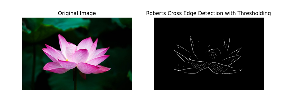

Scharr Edge Detection

Scharr edge detection is another method used to detect edges in digital images. It is an improvement over the Sobel operator. The Scharr operator consists of two 3x3 convolution kernels, one for approximating the horizontal gradient and the other for approximating the vertical gradient. These kernels are applied to the image to compute the gradient at each pixel, which highlights areas of rapid intensity change or edges.

The horizontal gradient kernel (Gx) is designed to approximate the rate of change of intensity in the horizontal direction, while the vertical gradient kernel (Gy) approximates the rate of change of intensity in the vertical direction. The Scharr kernels are as follows.

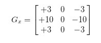
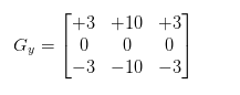
The cv.Scharr() method in OpenCV is a function used to calculate the first-order derivatives of an image using the Scharr operator. The Scharr operator is a derivative mask that is used to detect edges in an image. It is similar to the Sobel operator but is optimized to provide better rotational symmetry and more accurate edge detection for specific applications.

import cv2
import numpy as np
import matplotlib.pyplot as plt

def scharr_edge_detection(image):
    # Convert to grayscale
    gray_image = cv2.cvtColor(image, cv2.COLOR_BGR2GRAY)
    
    # Apply Scharr operator to find the x and y gradients
    Gx = cv2.Scharr(gray_image, cv2.CV_64F, 1, 0)
    Gy = cv2.Scharr(gray_image, cv2.CV_64F, 0, 1)
    
    # Compute the gradient magnitude
    gradient_magnitude = cv2.magnitude(Gx, Gy)
    
    return gradient_magnitude

def main():
    # Load the image
    image = cv2.imread('flower.jpg')
    
    if image is None:
        print("Error: Image not found.")
        return
    
    # Detect edges using Scharr operator
    edges = scharr_edge_detection(image)
    
    # Plot the results
    plt.figure(figsize=(15, 5))

    # Original Image
    plt.subplot(1, 2, 1)
    plt.imshow(cv2.cvtColor(image, cv2.COLOR_BGR2RGB))
    plt.title('Original Image')
    plt.axis('off')

    # Scharr Edge Detection
    plt.subplot(1, 2, 2)
    plt.imshow(edges, cmap='gray')
    plt.title('Scharr Edge Detection')
    plt.axis('off')

    plt.show()

if __name__ == "__main__":
    main()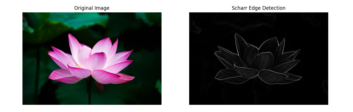

Gradient-Based Edge Detection

Gradient-based edge detection involves finding the gradient of the image intensity function. The gradient measures the rate of change of intensity, and edges are typically located where this rate of change is maximized. The primary tools used in gradient-based edge detection are gradient operators like Sobel, Prewitt, and Scharr.

Gaussian-Based Edge Detection

Gaussian-based edge detection involves smoothing the image with a Gaussian filter to reduce noise and then detecting edges, often using second-order derivatives like the Laplacian of Gaussian (LoG). This approach helps to find edges by locating zero-crossings of the second derivative of the image intensity function

Which Edge Detection Algorithm Should I Use?

Canny is the default: its smoothing, thinning, and hysteresis stages produce the cleanest usable edge maps, at the cost of two thresholds to tune. Use Sobel or Scharr when you need raw gradient magnitude and direction as features rather than a binary edge map, with Scharr preferred when edge orientation matters.

Use the Laplacian when precise localization via zero-crossings suits your task and noise is under control. Prewitt and Roberts Cross matter mostly for speed on constrained hardware and for understanding the field's history; on modern CPUs, Canny's overhead is rarely the bottleneck.

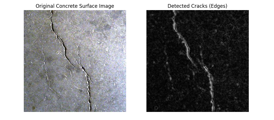
Edge Detection Example Use Case: Crack Detection in Concrete Structures

Concrete structures, such as bridges, buildings, and pavements, are susceptible to wear and tear over time due to environmental conditions, load stress, and other factors. Early detection of cracks in these structures is vital for maintenance and safety. Edge detection techniques can be used effectively to identify and analyze cracks - a critical task in structural health monitoring.

Here is an example to detect cracks in concrete structures.

import cv2
import numpy as np
import matplotlib.pyplot as plt

def preprocess_image(image):
    # Convert to grayscale
    gray_image = cv2.cvtColor(image, cv2.COLOR_BGR2GRAY)
    
    # Apply Gaussian blur to reduce noise
    blurred_image = cv2.GaussianBlur(gray_image, (5, 5), 0)
    
    return blurred_image

def detect_edges(image):
    # Apply Sobel edge detection
    sobelx = cv2.Sobel(image, cv2.CV_64F, 1, 0, ksize=3)
    sobely = cv2.Sobel(image, cv2.CV_64F, 0, 1, ksize=3)
    
    # Compute the gradient magnitude
    gradient_magnitude = np.sqrt(sobelx**2 + sobely**2)
    
    # Normalize the gradient magnitude to [0, 255]
    gradient_magnitude = np.uint8(255 * gradient_magnitude / np.max(gradient_magnitude))
    
    return gradient_magnitude
    
def main():
    # Read the image
    image = cv2.imread('concrete-shrinkage-crack.jpg')
    
    if image is None:
        print("Error: Image not found.")
        return
    
    # Preprocess the image
    preprocessed_image = preprocess_image(image)
    
    # Detect edges
    edges = detect_edges(preprocessed_image)
    
    # Plotting the results
    plt.figure(figsize=(10, 5))

    # Original Image
    plt.subplot(1, 2, 1)
    plt.imshow(cv2.cvtColor(image, cv2.COLOR_BGR2RGB))
    plt.title('Original Concrete Surface Image')
    plt.axis('off')

    # Detected Edges
    plt.subplot(1, 2, 2)
    plt.imshow(edges, cmap='gray')
    plt.title('Detected Cracks (Edges)')
    plt.axis('off')

    plt.show()

if __name__ == "__main__":
    main()

The following is the output of crack detection code.

Edge Detection vs. Learned Models

Classical edge detection is fast, deterministic, dependency-light, and needs zero training data. It is the right tool when the feature you want is the intensity change: measuring dimensions against a backlight, finding contours for shape analysis, or preprocessing before OCR or template matching.

It stops being the right tool when the question is what an edge means. A defect inspection system needs cracks but not texture; that requires a model trained on labeled examples, a segmentation or detection model like RF-DETR, which learns the semantic distinction a gradient cannot express.

In practice the two combine: Roboflow Workflows includes classical computer vision blocks (contours, thresholding, blur, contrast equalization) alongside model blocks, so a pipeline can use classical operations for preprocessing and measurement and a trained model for the judgment call. If your edge detection project keeps growing rules to suppress false edges, that is the signal to label a dataset and train.

Get Started

Run the snippets above on your own images to build intuition for what each operator sees. When your application needs to know which edges matter, create a free Roboflow account, label examples of the boundaries you care about, and train a model that finds them specifically.

What is edge detection in image processing?

A technique that locates object boundaries by finding places where pixel intensity changes sharply, producing an edge map used for segmentation, measurement, and feature extraction.

Which edge detection algorithm is best?

Canny, for most purposes: its multi-stage design produces thin, connected, low-noise edges. Sobel and Scharr are better when you need gradient values as features rather than a binary edge map.

What is the difference between Canny and Sobel?

Sobel is a single convolution step producing gradient magnitude; Canny builds on a Sobel-style gradient with smoothing, non-maximum suppression, and hysteresis thresholding to output clean edge lines. Sobel gives you the raw signal, Canny a finished edge map.

Is edge detection machine learning?

The classical algorithms are not; they are fixed mathematical operators with no training. Learned edge detectors exist, and more commonly the task that motivated edge detection (finding specific boundaries) is handled today by trained segmentation models.

When should I use a trained model instead of edge detection?

When the boundary you care about is defined by meaning rather than contrast: cracks but not texture, one product but not its neighbor. If you find yourself writing rules to filter unwanted edges, train a model on labeled examples instead.

Cite this Post

Use the following entry to cite this post in your research:

Timothy M. (May 6, 2026). Edge Detection in Image Processing: An Introduction. Roboflow Blog: https://blog.roboflow.com/edge-detection/