What is Thresholding in Image Processing? A Guide.

The article below was contributed by Timothy Malche, an assistant professor in the Department of Computer Applications at Manipal University Jaipur.

Thresholding in image processing is a technique used to create binary images from grayscale images. The process involves setting a threshold value and converting all pixels in the grayscale image to either black or white based on whether their intensity values are below or above the threshold. This technique is widely used in various applications such as image segmentation, object detection, and feature extraction.

Following are the different types of thresholding.

• Global Thresholding
• Local Thresholding

Suppose we have a grayscale image with pixel values ranging from 0 to 255. Assume a grayscale image represented by a 5x5 matrix of pixel values:

[
  [50, 100, 150, 200, 250],
  [60, 110, 160, 210, 240],
  [70, 120, 170, 220, 230],
  [80, 130, 180, 230, 220],
  [90, 140, 190, 240, 210]
]

We want to apply a global thresholding with a threshold value of 150. The process is as follows:

For each pixel value:

• If the value is >= 150, set it to 255 (white).
• If the value is < 150, set it to 0 (black).

Applying the threshold, the binary image becomes:

[
  [0,   0,   255, 255, 255],
  [0,   0,   255, 255, 255],
  [0,   0,   255, 255, 255],
  [0,   0,   255, 255, 255],
  [0,   0,   255, 255, 255]
]

Here, pixels with values less than 150 have been converted to 0 (black), and those with values 150 or greater have been converted to 255 (white).

Basic Terminology

Before we begin, let’s discuss a few terms that will be referenced in this guide.

• Binary Image: An image where each pixel is either black or white. After thresholding, an image typically becomes binary, where pixel values are 0 or 255.
• Histogram: In the context of thresholding, a histogram represents the distribution of pixel intensities in an image. It can be used to determine the optimal threshold value.
• Foreground and Background: In a binary image, the foreground is typically represented by white pixels (255) and the background by black pixels (0). Thresholding separates the foreground objects from the background.
• Segmentation: The process of partitioning an image into meaningful regions. Thresholding is a simple form of segmentation that divides an image into foreground and background regions.

Global Thresholding

In global thresholding, a single intensity value (threshold) is chosen. Pixels with intensity values greater than this threshold are classified as foreground (usually assigned a value of 255, which is white in grayscale), and those with intensity values lower than the threshold are classified as background (usually assigned a value of 0, which is black in grayscale).

Given a grayscale image 𝐼, the thresholding operation can be defined as:

​Where:

• 𝑇 is the threshold value, and;
• (𝑥,𝑦) are the coordinates of a pixel in the image.

The choice of the threshold value 𝑇 is crucial for the effectiveness of the segmentation. There are several methods to choose 𝑇:

• Manual Selection
• Histogram Analysis
• Otsu's Method

Manual Selection

In this we manually choose a threshold value based on visual inspection. For example, if the threshold is 128:

• Pixels >= 128 become 255.
• Pixels < 128 become 0.

In OpenCV, thresholding can be implemented using cv.threshold() function and specifying the manual threshold value as the second parameter to function. Here’s the code.

import cv2
import numpy as np
import matplotlib.pyplot as plt

# Load the image
color_image = cv2.imread('flower.jpg', cv2.IMREAD_COLOR)

# convert to grayscale image
grayscale_image = cv2.cvtColor(color_image, cv2.COLOR_BGR2GRAY)

# Manual thresholding
threshold_value = 128  # Example manual threshold value
_, binary_image = cv2.threshold(grayscale_image, threshold_value, 255, cv2.THRESH_BINARY)

# Display the original and thresholded images
plt.figure(figsize=(15, 5))

plt.subplot(1, 3, 1)
plt.title('Original Image')
plt.imshow(color_image, cmap='gray')
plt.axis('off')

plt.subplot(1, 3, 2)
plt.title('Grayscale Image')
plt.imshow(grayscale_image, cmap='gray')
plt.axis('off')

plt.subplot(1, 3, 3)
plt.title(f'Global Thresholding (T={threshold_value})')
plt.imshow(binary_image, cmap='gray')
plt.axis('off')
plt.show()

Our script generates the following output:

Global Image Thresholding using Manual Thresholding

Histogram Analysis 

Analyze the histogram of the image's pixel intensities. A common approach is to choose threshold 𝑇 at the valley between the peaks of the histogram representing the foreground and background. Here the following steps are used.

• Load the image and convert to grayscale image.
• Compute the histogram of the grayscale image using np.histogram.
• Compute the cumulative distribution function (CDF) of the histogram.
• Normalize the CDF to the range [0, 1] for easier threshold determination.
• Find the threshold value by identifying the point in the CDF where it exceeds 0.5 (this is a simplistic approach; you can adjust this thresholding logic based on your requirements).
• Create a binary thresholded image where pixel values above the threshold are set to 255 (white), and below or equal are set to 0 (black).

import cv2
import numpy as np
import matplotlib.pyplot as plt

# Load an image
color_image = cv2.imread('flower.jpg', cv2.IMREAD_COLOR)

# Convert to grayscale image
grayscale_image = cv2.cvtColor(color_image, cv2.COLOR_BGR2GRAY)

# Calculate histogram
histogram, bins = np.histogram(grayscale_image.flatten(), 256, [0,256])

# Calculate cumulative distribution function (CDF)
cdf = histogram.cumsum()

# Normalize CDF to range [0, 1]
cdf_normalized = cdf / cdf.max()

# Find the threshold value (simplest method: midpoint thresholding)
threshold_value = np.argmax(cdf_normalized > 0.5)

# Apply thresholding to create a binary image
thresholded_image = np.zeros_like(grayscale_image)
thresholded_image[grayscale_image > threshold_value] = 255

# Plotting
plt.figure(figsize=(15, 8))

# Original image
plt.subplot(2, 3, 1)
plt.imshow(cv2.cvtColor(color_image, cv2.COLOR_BGR2RGB))
plt.title('Original Image')
plt.axis('off')

# Grayscale image
plt.subplot(2, 3, 2)
plt.imshow(grayscale_image, cmap='gray')
plt.title('Grayscale Image')
plt.axis('off')

# Thresholded image
plt.subplot(2, 3, 3)
plt.imshow(thresholded_image, cmap='gray')
plt.title('Thresholded Image')
plt.axis('off')

# Histogram
plt.subplot(2, 3, 4)
plt.hist(grayscale_image.flatten(), bins=256, range=[0,256], color='gray', alpha=0.7)
plt.axvline(x=threshold_value, color='r', linestyle='--', linewidth=1.5)
plt.title('Histogram')
plt.xlabel('Pixel Intensity')
plt.ylabel('Frequency')

# CDF
plt.subplot(2, 3, 5)
plt.plot(cdf_normalized, color='b')
plt.title('CDF')
plt.xlabel('Pixel Intensity')
plt.ylabel('CDF Value')

plt.tight_layout()
plt.show()

Below is the output of the code:

Image Thresholding using Histogram Analysis

Otsu's Method

Otsu thresholding is an automatic thresholding technique used in image processing to separate an image into foreground and background. It does so by finding an optimal threshold value that minimizes the intra-class variance (the variance within each of the two classes, foreground and background) or equivalently maximizes the inter-class variance (the variance between the two classes). Let's use a simple example with grayscale pixel values to explain intra-class and inter-class variance. Imagine you have a small grayscale image with the following pixel values:

[
  [10, 10, 12, 12],
  [10, 10, 12, 12],
  [200, 200, 220, 220],
  [200, 200, 220, 220]
]

In this example, the pixel values are either low (around 10-12) or high (around 200-220). Our goal is to separate these two groups using thresholding.

Intra-class variance measures how similar the pixel values are within each group (class). If we choose a threshold, say 100, to separate the pixels into two classes (background and foreground):

• Background Class: Pixels below the threshold (10, 10, 12, 12, 10, 10, 12, 12)
• Foreground Class: Pixels above the threshold (200, 200, 220, 220, 200, 200, 220, 220)

The intra-class variance for each class is the measure of the spread of the pixel values within that class.

• Background Class Variance: All values are close to each other (10-12), so the variance is low.
• Foreground Class Variance: All values are close to each other (200-220), so the variance is also low.

When intra-class variance is low, it means that within each class, the pixel values are very similar.

Inter-class variance measures how different the two classes are from each other. It looks at the difference between the average values (means) of the two classes.

• Mean of Background Class: The average of (10, 10, 12, 12, 10, 10, 12, 12)
• Mean of Foreground Class: The average of (200, 200, 220, 220, 200, 200, 220, 220)

If the difference between these means is large, the inter-class variance is high. In our case, the mean of the background is around 11, and the mean of the foreground is around 210, making the inter-class variance high.

The Otsu’s method is particularly useful for images with a bimodal histogram, where two distinct peaks represent the background and the foreground. The idea behind this method is to separate the image histogram into two clusters using a threshold that minimizes the weighted variance of these classes. To the intra-class variance for all possible threshold 𝑡 values the computation can be described using the equation:

where 𝑤₁(𝑡) and 𝑤₂(𝑡) are the probabilities of the two classes divided by the threshold 𝑡, which ranges from 0 to 255 inclusively. σ₁²(t) and σ₂²(t) are the variances of the two classes at threshold 𝑡.

To apply Otsu’s method we simply need to use OpenCV threshold() function with set THRESH_OTSU flag:

import cv2
import numpy as np
import matplotlib.pyplot as plt

# Load the image
color_image = cv2.imread('flower.jpg', cv2.IMREAD_COLOR)

# convert to grayscale image
grayscale_image = cv2.cvtColor(color_image, cv2.COLOR_BGR2GRAY)

# Apply Otsu's thresholding
_, otsu_binary_image = cv2.threshold(grayscale_image, 0, 255, cv2.THRESH_BINARY + cv2.THRESH_OTSU)
otsu_threshold = cv2.threshold(grayscale_image, 0, 255, cv2.THRESH_BINARY + cv2.THRESH_OTSU)[0]
# Display the original, grayscale and thresholded imagesplt.figure(figsize=(15, 5))
plt.subplot(1, 3, 1)
plt.title('Original Image')
plt.imshow(color_image, cmap='gray')
plt.axis('off')

plt.subplot(1, 3, 2)
plt.title('Grayscale Image')
plt.imshow(grayscale_image, cmap='gray')
plt.axis('off')

plt.subplot(1, 3, 3)
plt.title(f"Otsu's Thresholding (T={int(otsu_threshold)})")
plt.imshow(otsu_binary_image, cmap='gray')
plt.axis('off')

plt.show()

Below is the output of the code:

Local Thresholding

Local thresholding is a technique used to binarize an image by determining the threshold value locally for each pixel based on the characteristics of the surrounding neighborhood. Unlike global thresholding, which uses a single threshold value for the entire image, adaptive thresholding calculates the threshold for smaller regions of the image, allowing for variations in lighting and contrast within the image. This makes it particularly useful for images with non-uniform lighting or shadows.

There are two main types of adaptive thresholding methods, adaptive mean thresholding and adaptive Gaussian thresholding.

Adaptive Mean Thresholding

In adaptive mean thresholding, the threshold value for each pixel is determined by the mean of the pixel values in the local neighborhood (a small window around the pixel). A constant value is then subtracted from this mean to get the final threshold value.

Here is how the method works. For each pixel at coordinates (𝑥,𝑦) in the image, the threshold value 𝑇(𝑥,𝑦) is calculated using he mean 𝜇(𝑥,𝑦) of the pixel intensities within a local neighborhood. The formula for the threshold is:

Where:

• 𝜇(𝑥,𝑦) is the mean intensity of the local neighborhood.
• 𝐶 is a constant value subtracted from the mean to fine-tune the thresholding.

Adaptive Gaussian Thresholding

In adaptive Gaussian thresholding, the threshold value for each pixel is determined by a weighted sum of the pixel values in the local neighborhood, where the weights are a Gaussian window (a window with a Gaussian distribution).

Here is how it works. For each pixel at coordinates (𝑥,𝑦) in the image, the threshold value 𝑇(𝑥,𝑦) is calculated using the weighted sum of the pixel intensities within a local neighborhood, where the weights follow a Gaussian distribution. The formula for the threshold is:

Where:

• The Gaussian-weighted sum is computed using a Gaussian window centered at (𝑥,𝑦).
• 𝐶 is a constant value subtracted from the Gaussian-weighted sum to fine-tune the thresholding.

OpenCV provides the cv.adaptiveThreshold() method for adaptive thresholding which takes cv.ADAPTIVE_THRESH_MEAN_C parameter for adaptive mean thresholding and cv.ADAPTIVE_THRESH_GAUSSIAN_C parameter for adaptive gaussian as one of its parameters.

import cv2
import matplotlib.pyplot as plt

# Load the original color image
color_image = cv2.imread('flower.jpg')

# Convert the color image to grayscale
gray_image = cv2.cvtColor(color_image, cv2.COLOR_BGR2GRAY)

# Apply Adaptive Mean Thresholding
adaptive_mean = cv2.adaptiveThreshold(gray_image, 255, cv2.ADAPTIVE_THRESH_MEAN_C, 
                                      cv2.THRESH_BINARY, 11, 2)

# Apply Adaptive Gaussian Thresholding
adaptive_gaussian = cv2.adaptiveThreshold(gray_image, 255, cv2.ADAPTIVE_THRESH_GAUSSIAN_C, 
                                          cv2.THRESH_BINARY, 11, 2)

# Display the original, grayscale, and thresholded images
titles = ['Original Image', 'Grayscale Image', 'Adaptive Mean Thresholding', 'Adaptive Gaussian Thresholding']
images = [color_image, gray_image, adaptive_mean, adaptive_gaussian]

plt.figure(figsize=(15, 10))
for i in range(4):
    plt.subplot(2, 2, i+1)
    if i == 0:
        plt.imshow(cv2.cvtColor(images[i], cv2.COLOR_BGR2RGB))  # Convert BGR to RGB for displaying correctly with matplotlib
    else:
        plt.imshow(images[i], cmap='gray')
    plt.title(titles[i])
    plt.xticks([]), plt.yticks([])
plt.show()

Local Image Thresholding using Adaptive Mean and Gaussian Thresholding

Apart from Adaptive Mean and Gaussian Thresholding the other popular local thresholding techniques are using Niblack’s method, Sauvola's and Bernsen’s method that we are going to discuss here.

Niblack's Method

Niblack's method is a local thresholding technique used in image processing to segment an image into foreground and background regions. It computes the threshold for each pixel based on the mean and standard deviation of the pixel intensities in a local neighborhood.

Here is how this method work. For each pixel at coordinates (𝑥,𝑦) in the image, the threshold value 𝑇(𝑥,𝑦) is calculated using the mean 𝜇(𝑥,𝑦) and standard deviation 𝜎(𝑥,𝑦) of the pixel intensities within a window (or neighborhood) centered around the pixel. The formula for the threshold is:

Where:

• 𝜇(𝑥,𝑦) is the mean intensity of the local neighborhood.
• 𝜎(𝑥,𝑦) is the standard deviation of the local neighborhood.
• 𝑘 is a user-defined parameter that adjusts the level of thresholding.

OpenCV does not provide any direct method for Niblack method so we will use scikit-image library for this thresholding. First, install the library:

pip install scikit-image

Then, use the following code:

import matplotlib.pyplot as plt
import cv2
from skimage.filters import threshold_niblack

# Read the color image using OpenCV
image_color = cv2.imread('flower.jpg', cv2.IMREAD_COLOR)

# Convert color image to grayscale for processing
image_gray = cv2.cvtColor(image_color, cv2.COLOR_BGR2GRAY)

# Apply Niblack thresholding
window_size = 25
thresh_niblack = threshold_niblack(image_gray, window_size=window_size, k=0.8)
binary_niblack = image_gray > thresh_niblack

# Plotting
plt.figure(figsize=(12, 6))

# Original Color Image
plt.subplot(1, 3, 1)
plt.imshow(cv2.cvtColor(image_color, cv2.COLOR_BGR2RGB))
plt.title('Original Color')
plt.axis('off')

# Original Grayscale Image
plt.subplot(1, 3, 2)
plt.imshow(image_gray, cmap=plt.cm.gray)
plt.title('Original Grayscale')
plt.axis('off')

# Niblack Threshold Image
plt.subplot(1, 3, 3)
plt.imshow(binary_niblack, cmap=plt.cm.gray)
plt.title('Niblack Threshold')
plt.axis('off')

plt.tight_layout()
plt.show()

Following will be the output when you run the code.

Niblack Threshold

Sauvola's Method

Sauvola's method is an improvement over Niblack's method for adaptive local thresholding. It is designed to handle images with varying illumination and improve the binarization of images, particularly for document images containing text and background noise. This method adapts the threshold based on the local mean and standard deviation but introduces a dynamic range parameter to handle variations more effectively.

Here's how the method works. For each pixel at coordinates (𝑥,𝑦) in the image, the threshold value 𝑇(𝑥,𝑦) is calculated using the mean 𝜇(𝑥,𝑦) and standard deviation 𝜎(𝑥,𝑦) of the pixel intensities within a local neighborhood. The formula for the threshold is:

Where:

• 𝜇(𝑥,𝑦) is the mean intensity of the local neighborhood.
• 𝜎(𝑥,𝑦) is the standard deviation of the local neighborhood.
• 𝑘 is a user-defined parameter, which adjusts the level of thresholding.
• 𝑅 is the dynamic range of standard deviation, usually set to 128 for an 8-bit grayscale image.

Here’s the code to calculate Sauvoia threshold using scikit-image library.

import cv2
import numpy as np
import matplotlib.pyplot as plt
from skimage.filters import threshold_sauvola
from skimage import io, color

# Load the color image
image_color = io.imread('flower.jpg')

# Convert color image to grayscale
image_gray = color.rgb2gray(image_color)

# Apply Sauvola's method using skimage
window_size = 25
thresh_sauvola = threshold_sauvola(image_gray, window_size=window_size)

binary_sauvola = image_gray > thresh_sauvola

# Plotting
plt.figure(figsize=(12, 6))

# Original Color Image
plt.subplot(1, 3, 1)
plt.imshow(image_color)
plt.title('Original')
plt.axis('off')

# Grayscale Image
plt.subplot(1, 3, 2)
plt.imshow(image_gray, cmap='gray')
plt.title('Grayscale')
plt.axis('off')

# Sauvola Threshold Image
plt.subplot(1, 3, 3)
plt.imshow(binary_sauvola, cmap='gray')
plt.title('Sauvola Threshold')
plt.axis('off')

plt.tight_layout()
plt.show()

This will be the output when you run the code:

Bernsen’s Method

The Bernsen method is a local thresholding technique used in image processing to segment an image into foreground and background regions. This method works based on the contrast of an image. The threshold is set at the midrange value, which is the mean of the minimum 𝐼_low(𝑖,𝑗) and maximum 𝐼_high(𝑖,𝑗) gray values in a local window of suggested size 𝑤. However, if the contrast 

is below a certain contrast threshold 𝑘, the pixels within the window may be set to background or to foreground according to the class that most suitably describes the window. This algorithm is dependent on the value of 𝑘 and also on the size of the window.

Where:

• I(𝑖+𝑚,𝑗+𝑛): This represents the intensity value of a pixel at coordinates (𝑖+𝑚,𝑗+𝑛)
• max_𝑤[𝐼(𝑖+𝑚,𝑗+𝑛)]: This is the maximum intensity value within the local window 𝑤 centered around the pixel (𝑖,𝑗).
• min_𝑤[𝐼(𝑖+𝑚,𝑗+𝑛)]: This is the minimum intensity value within the local window 𝑤 centered around the pixel (𝑖,𝑗).
• 0.5: This factor takes the average (or midrange) of the maximum and minimum intensity values within the local window

For the example of Bernsen’s method, we will use mahotas.thresholding.bernsen() function from Mahotas library (a computer vision library for Python for image processing tasks). You can install library with following command.

pip install mahotas

Following is the code for thresholding using Bernsen method.

import mahotas
import cv2
import numpy as np
import matplotlib.pyplot as plt

# Load the color image
color_image = cv2.imread('flower.jpg')
# Convert the color image to grayscale
grayscale_image = cv2.cvtColor(color_image, cv2.COLOR_BGR2GRAY)

# Apply Bernsen's method using Mahotas
window_size = 5
contrast_threshold = 200
bernsen_result = mahotas.thresholding.bernsen(grayscale_image, window_size, contrast_threshold)

# Display the original color image, grayscale image, and thresholded image
titles = ['Original Color Image', 'Grayscale Image', 'Bernsen Thresholding (Mahotas)']
images = [cv2.cvtColor(color_image, cv2.COLOR_BGR2RGB), grayscale_image, bernsen_result]

plt.figure(figsize=(15, 5))
for i in range(3):
    plt.subplot(1, 3, i+1)
    plt.imshow(images[i], cmap='gray' if i > 0 else None)
    plt.title(titles[i])
    plt.xticks([]), plt.yticks([])
plt.show()

Running the code will generate following output.

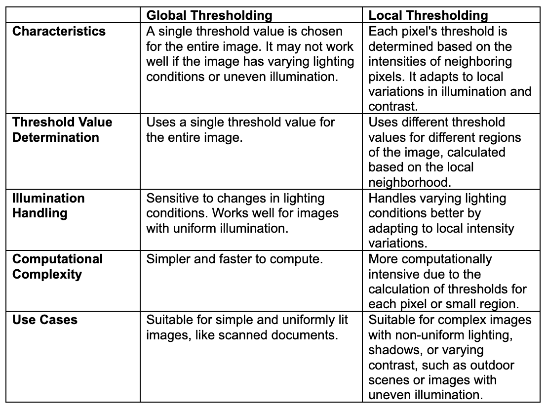
Global vs Local Thresholding

In this section, we explore the fundamental distinctions between global and local thresholding methods, and help determine the optimal approach for the given task.

Example of Global Thresholding vs Local Thresholding (Source)

Thresholding Operations

OpenCV offers various types of thresholding methods, specified by the fourth parameter of the cv.thresholding() and cv.adaptiveThreshold() functions. The basic thresholding method can be performed using the type cv.THRESH_BINARY. The various thresholding methods represent different threshold operations. The following table shows different threshold operations and which operation works with which function.

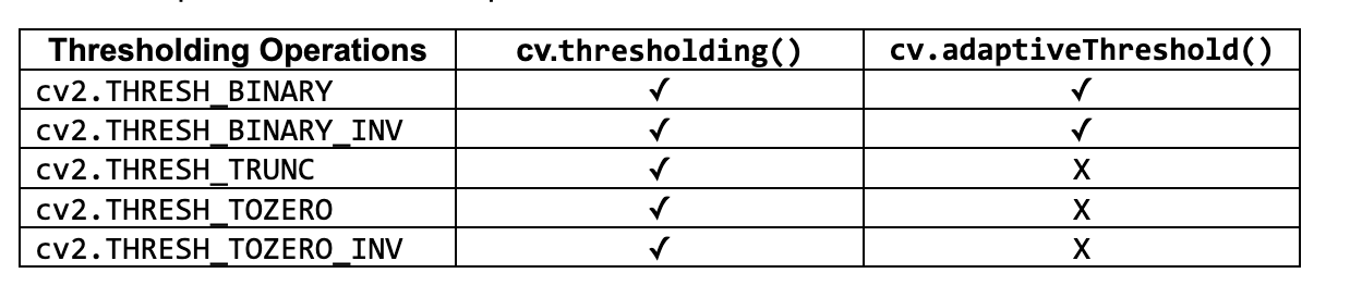
✓ - Can be used

X – Can not be used

To understand the working of each of these operations, imagine you have a grayscale image where pixel values range from 0 (black) to 255 (white). Let's say we set a threshold value of 127, then each of these operation work as following:

• cv2.THRESH_BINARY: If a pixel's value is greater than 127, it is set to 255 (white). If it is less than or equal to 127, it is set to 0 (black).
• cv2.THRESH_BINARY_INV: If a pixel's value is greater than 127, it is set to 0 (black). If it is less than or equal to 127, it is set to 255 (white).
• cv2.THRESH_TRUNC: If a pixel's value is greater than 127, it is set to 127. If it is less than or equal to 127, it remains unchanged.
• cv2.THRESH_TOZERO: If a pixel's value is greater than 127, it remains unchanged. If it is less than or equal to 127, it is set to 0 (black).
• cv2.THRESH_TOZERO_INV: If a pixel's value is greater than 127, it is set to 0 (black). If it is less than or equal to 127, it remains unchanged.

import cv2
import numpy as np
import matplotlib.pyplot as plt

# Load the grayscale image
image = cv2.imread('flower.jpg', cv2.IMREAD_GRAYSCALE)

# Define the threshold value and maximum value
thresh = 127
maxVal = 255

# Apply different thresholding types
_, binary = cv2.threshold(image, thresh, maxVal, cv2.THRESH_BINARY)
_, binary_inv = cv2.threshold(image, thresh, maxVal, cv2.THRESH_BINARY_INV)
_, trunc = cv2.threshold(image, thresh, maxVal, cv2.THRESH_TRUNC)
_, tozero = cv2.threshold(image, thresh, maxVal, cv2.THRESH_TOZERO)
_, tozero_inv = cv2.threshold(image, thresh, maxVal, cv2.THRESH_TOZERO_INV)

# Display the original and thresholded images
titles = ['Original Image', 'THRESH_BINARY', 'THRESH_BINARY_INV', 'THRESH_TRUNC', 'THRESH_TOZERO', 'THRESH_TOZERO_INV']
images = [image, binary, binary_inv, trunc, tozero, tozero_inv]

plt.figure(figsize=(10, 10))
for i in range(6):
    plt.subplot(3, 2, i+1)
    plt.imshow(images[i], cmap='gray')
    plt.title(titles[i])
    plt.xticks([]), plt.yticks([])
plt.show()

Following is the output of above code.

These different methods allow to manipulate images in various ways, which can be useful depending on the task at hand, such as highlighting certain features, improving contrast, or preparing images for further processing like edge detection or object recognition.

Conclusion

Thresholding is a fundamental image processing technique that separates objects from the background by setting a pixel intensity cutoff. Thresholding can be performed globally or locally to accommodate uniform or varying lighting conditions.

Global methods, like Otsu's, work well for distinct bimodal histograms, while local methods adapt to non-uniform illumination. We covered in depth the global thresholding method and explored several local thresholding methods, including mean, Gaussian, Bernsen, Niblack, and Sauvola, each with unique approaches to setting thresholds based on local image properties.

We have seen how to practically implement using OpenCV, Scikit-Image and Mahotas libraries. The thresholding technique can be applied to numerous practical use cases, such as this implementation of Otsu’s method in Google Earth Engine, and in applications such as object detection, segmentation, document binarization, and medical imaging.