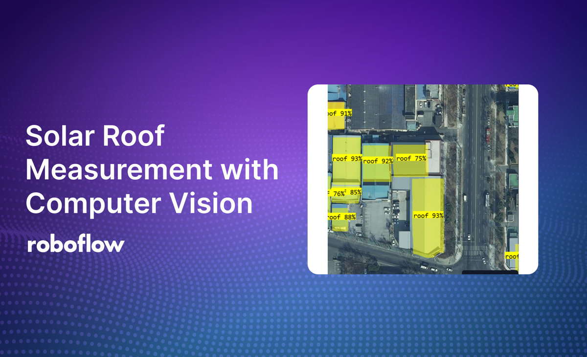
The transition to renewable energy sources has accelerated the demand for solar panel installations. For solar businesses and installers, accurately estimating the roof surface area is crucial for planning, costing, and optimizing the number of solar panels that can be installed on a specific house.
Traditional methods of roof measurement can be time-consuming and labor-intensive. However, with advancements in computer vision and the availability of high-resolution aerial imagery, it's now possible to automate this process efficiently.
This guide will walk you through how to use computer vision to measure the surface area of roofs from aerial images, and how to estimate the area for solar panel installation.
In this article, we’ll explore how to detect roof areas in aerial images taken from drones. We will train an instance segmentation model which will provide roof area coordinates.
These coordinates are then used to calculate the surface area in pixel using shoelace algorithm and convert this pixel area to real-world units using the Ground Sample Distance (GSD).
Building the Roof Area Measurement System
Let us explore the steps for building the roof area measurement system.
Step #1: Training Computer Vision Model
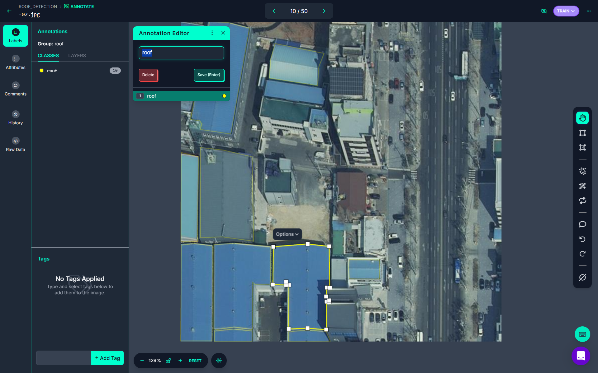
Our first step would be training Computer Vision Model to detect the roof area in aerial images taken from drones. This requires collecting images of roof and annotating it using Roboflow’s annotation tool. The following is an example of annotating roof area in image using polygon annotation tool.
After annotating all roofs in image, the annotation looks like following.
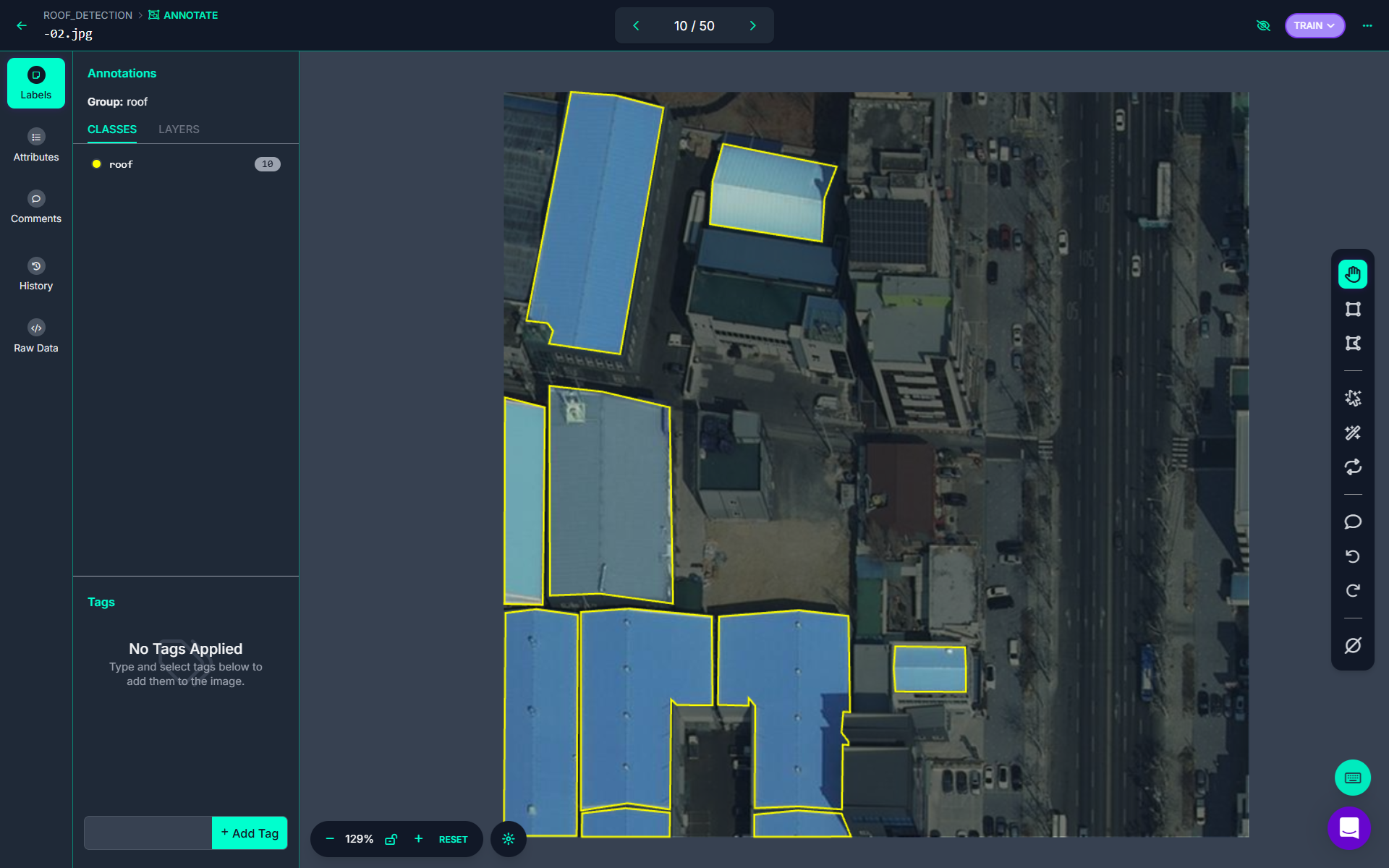
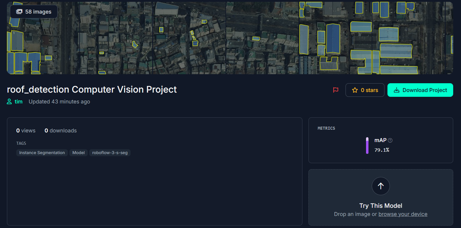
For this project, it's essential to obtain the polygon coordinates in the image, as roofs often do not have a rectangular structure. The trained roof detection model provides both the roof area and its corresponding polygon points.
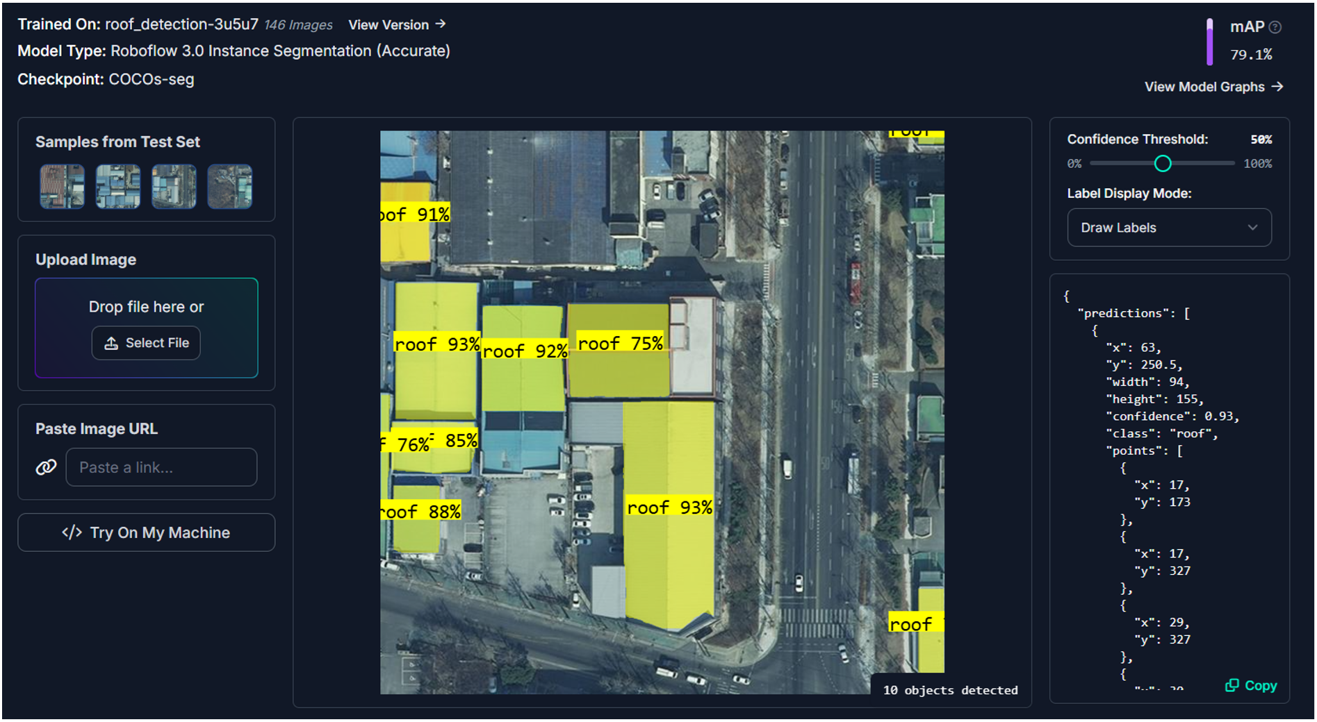
The roof detection model, as shown in the image above, generates polygon points for each roof, which can then be utilized for further analysis.
Step #2: Data Preparation
The output from the roof detection model is structured as a JSON-like dictionary containing:
- Coordinates: Each roof is represented by a series of x, y points defining its polygon. Polygons are used to calculate and visualize roof areas.
- Metadata: Information such as confidence score, detection ID, width, and height of the detected roof.
{'inference_id': 'a34c6485-1beb-449a-a575-0aa176170a8e',
 'time': 0.17079827900033706,
 'image': {'width': 640, 'height': 640},
 'predictions': [{'x': 281.5,
   'y': 34.5,
   'width': 79.0,
   'height': 69.0,
   'confidence': 0.924842357635498,
   'class': 'roof',
   'points': [{'x': 265.0, 'y': 0.0},
    {'x': 265.0, 'y': 3.0},
    {'x': 264.0, 'y': 4.0},
    {'x': 264.0, 'y': 6.0},

    . . .

    {'x': 319.0, 'y': 0.0}],
   'class_id': 0,
   'detection_id': '30876aa3-e702-46ec-bca8-5f7cc042bcdd'}]}
This data needs to be prepared for input to the roof measurement script. The following inference will prepare the data and store it in a variable data which will be used later.
# Import the Roboflow Inference SDK
from inference_sdk import InferenceHTTPClient

# Initialize the client
CLIENT = InferenceHTTPClient(
    api_url="https://detect.roboflow.com",
    api_key="YOUR_API_KEY"  # Replace with your API key
)

# Infer on a local image
result = CLIENT.infer("roof.jpg", model_id="roof_detection-3u5u7/2")

# Store the result in the `data` variable
data = {
    "predictions": [
        {
            "x": prediction["x"],
            "y": prediction["y"],
            "width": prediction["width"],
            "height": prediction["height"],
            "confidence": prediction["confidence"],
            "class": prediction["class"],
            "points": prediction["points"],
            "class_id": prediction["class_id"],
            "detection_id": prediction["detection_id"],
        }
        for prediction in result.get("predictions", [])
    ]
}

# Print the  data
print(data)
The result is fetched and stored in the variable data in the following form.
{
    "predictions": [
        {
            "points": [{"x": 17, "y": 173}, {"x": 17, "y": 327}, ...],
            "confidence": 0.93,
            "detection_id": "6cc33b65-5148-40cd-a310-7c432a98751a",
            ...
        },
        ...
    ]
}
This data is passed to the analysis pipeline.
Step #3: Ground Sample Distance (GSD) Calculation
The GSD determines the real-world size of each pixel in the image. This value is essential for converting areas calculated in pixel units to square meters. In the code the GSD is set as following:
gsd = 0. 0959 # meters per pixel
Calculation of GSD is crucial for the project as it will help determine the actual roof area.
What is GSD?
GSD is a concept in remote sensing, aerial photography, and satellite imaging. GSD refers to the physical distance on the ground that each pixel in a digital image represents. In other words, it's a measure of the resolution of an aerial or satellite image, indicating how much real-world area is captured by a single pixel.
GSD defines the real-world size represented by each pixel in an image. GSD measures the distance between the centers of two consecutive pixels on the ground. For example, a GSD of 5 centimeters per pixel means that each pixel in the image corresponds to a 5 cm × 5 cm area on the Earth's surface.
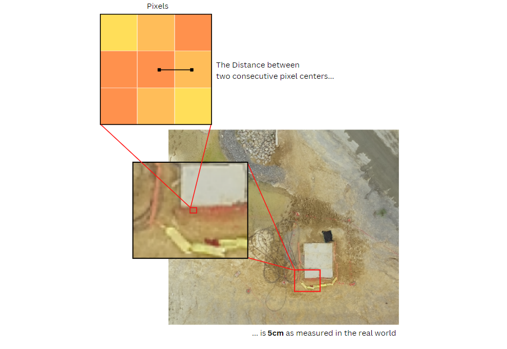
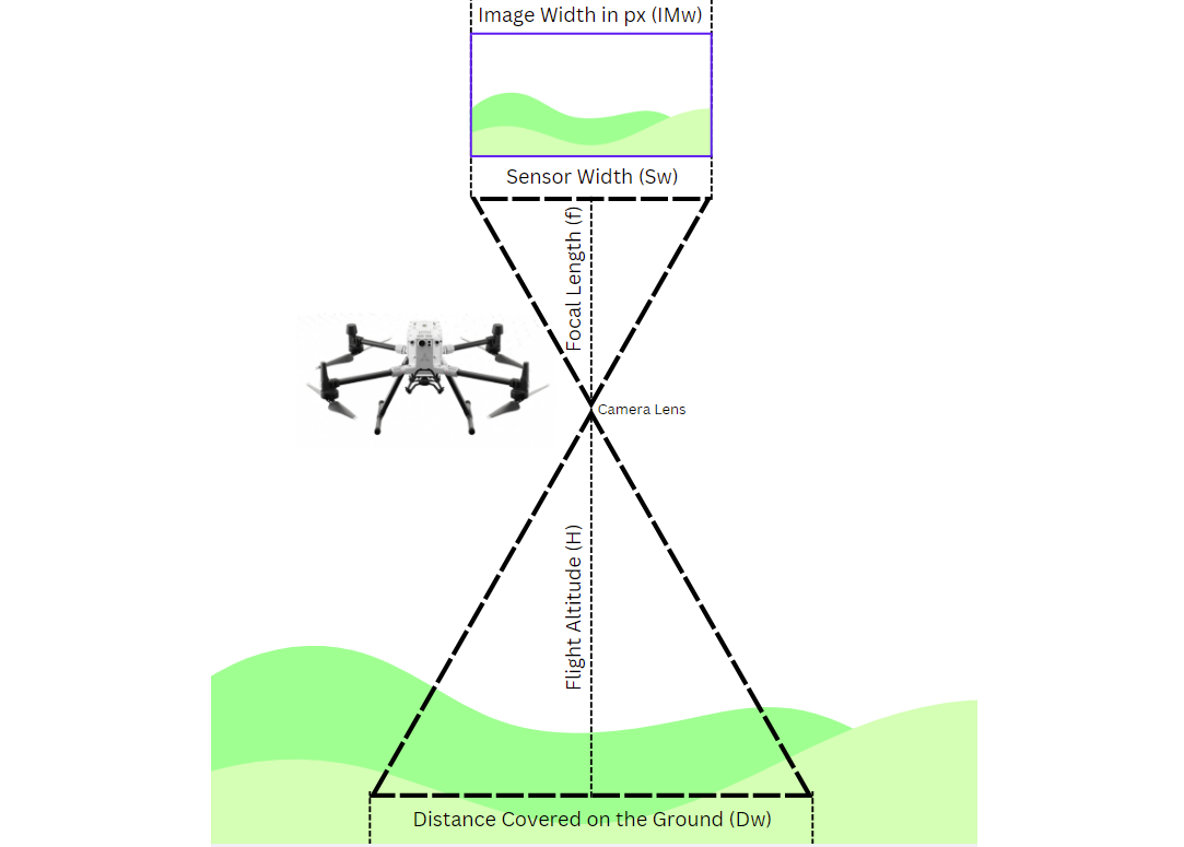
The GSD is influenced by factors such as the camera's sensor size, focal length, flight altitude, and image dimensions. The general formula to calculate GSD is:

Where:
- Sensor Width: Physical width of the camera's sensor (e.g., in millimeters).
- Flight Altitude: Height of the camera above the ground during image capture (e.g., in meters).
- Focal Length: Distance between the camera lens and the sensor (e.g., in millimeters).
- Image Width: Number of pixels along the image's width.
How is GSD Calculated?
Here's the GSD calculated. We assume that images are taken from the DJI Mavic Air 2 with the following parameters:
- Sensor Width: 13.2 mm
- Image Width: 5472 pixels
- Focal Length: 8.8 mm
- Flight Altitude: 350 meters
To calculate GSD following algorithm is used which gives actual ground distance covered by each pixel in your image.
def calculate_gsd(sensor_width_mm, image_width_px, focal_length_mm, flight_altitude_m):
    """
    Calculate Ground Sample Distance (GSD) in meters per pixel.

    Parameters:
        sensor_width_mm (float): Sensor width in millimeters.
        image_width_px (int): Image width in pixels.
        focal_length_mm (float): Focal length of the lens in millimeters.
        flight_altitude_m (float): Altitude of the camera above the ground in meters.

    Returns:
        float: GSD in meters per pixel.
    """
    gsd = (sensor_width_mm * flight_altitude_m) / (focal_length_mm * image_width_px)
    return gsd

# Example values
sensor_width_mm = 13.2  # Width of the sensor in mm (e.g., DJI Phantom 4 Pro)
image_width_px = 5472  # Image width in pixels
focal_length_mm = 8.8  # Focal length in mm
flight_altitude_m = 350  # Altitude in meters

# Calculate GSD
gsd = calculate_gsd(sensor_width_mm, image_width_px, focal_length_mm, flight_altitude_m)
print(f"Ground Sample Distance (GSD): {gsd:.4f} meters per pixel")
It will give following output
Ground Sample Distance (GSD): 0.0959 meters per pixel
This means that each pixel in your image represents a 9.59 cm × 9.59 cm area on the ground. The GSD value of 0.0959 meters per pixel means that each pixel in the image represents a square area of 0.0959×0.0959 = 0.00919681 m2.
Step #4: Area Calculation Using the Shoelace Algorithm
To compute the area of each roof polygon, the Shoelace algorithm is used.
What is the Shoelace Algorithm?
The Shoelace Algorithm, also known as the Shoelace Formula or Gauss's Area Formula, is a mathematical method used to calculate the area of a simple polygon when the coordinates of its vertices are known. It's called the "shoelace" algorithm because the calculation involves cross-multiplying coordinates in a manner that visually resembles the lacing of a shoe.
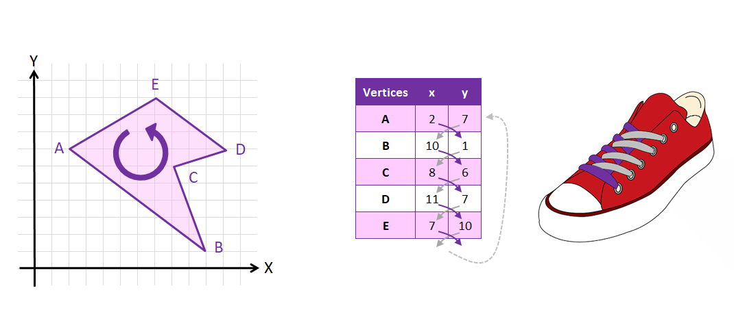
For a polygon with vertices (x1,y1),(x2,y2),…,(xn,yn) the area A of polygon P is calculated as:

In the code the following implementation of algorithm calculates the area of a polygon based on its vertex coordinates.
# Function to calculate polygon area using the Shoelace formula
def calculate_polygon_area(points):
    x_coords = [p['x'] for p in points]
    y_coords = [p['y'] for p in points]
    n = len(points)
    area = 0.5 * abs(
        sum(
            x_coords[i] * y_coords[(i + 1) % n] -
            y_coords[i] * x_coords[(i + 1) % n]
            for i in range(n)
        )
    )
    return area
Calling the above function, gives the area in pixel.
area_px = calculate_polygon_area(points)
Step #5: Convert Area to Physical Units
Once the polygon area is computed in pixels, it is converted to square meters using the GSD:
area_m2 = area_px * (gsd ** 2)
This step ensures that the results are meaningful for real-world applications.
Step #6: Visualization
Finally visualize the roof polygons on a Matplotlib plot. To distinguish each roof, assign a unique random color by generating random colors.
def random_color():
    return "#{:06x}".format(random.randint(0, 0xFFFFFF))
For each detected roof, plot each polygon. First, polygon points are extracted and plot the polygon using Matplotlib's Polygon patch. The random color is used as the fill color.
polygon = patches.Polygon(
    np.column_stack((x_coords, y_coords)),
    closed=True,
    edgecolor='black',
    facecolor=color,
    alpha=0.8
)
ax.add_patch(polygon)
Each roof is annotated by adding a text annotation at the polygon's centroid which display the roof's area in square meters.
centroid_x = np.mean(x_coords)
centroid_y = np.mean(y_coords)
ax.text(
    centroid_x, centroid_y,
    f"Roof-{idx+1}\nArea: {area_m2:.2f} m²",
    color='white',
    fontsize=10,
    weight='bold',
    ha='center',
    va='center',
    bbox=dict(facecolor='black', alpha=0.6, edgecolor='none')
)
Below is the full code:
data variable that we prepared in the Step #2: Data Preparation.import matplotlib.pyplot as plt
import matplotlib.patches as patches
import numpy as np
import random
# GSD value (in meters per pixel)
gsd = 0.0959 # Each pixel represents 0.0219 meters
# Function to calculate polygon area using the Shoelace formula
def calculate_polygon_area(points):
x_coords = [p['x'] for p in points]
y_coords = [p['y'] for p in points]
n = len(points)
area = 0.5 * abs(
sum(
x_coords[i] * y_coords[(i + 1) % n] -
y_coords[i] * x_coords[(i + 1) % n]
for i in range(n)
)
)
return area
# Generate a random color
def random_color():
return "#{:06x}".format(random.randint(0, 0xFFFFFF))
# Create a plot for visualization
fig, ax = plt.subplots(figsize=(18, 14))
ax.set_title("Roof Areas in Physical Units")
ax.set_aspect('equal')
# Iterate through predictions to calculate and visualize
for idx, prediction in enumerate(data["predictions"]):
# Extract points
points = prediction["points"]
x_coords = [p['x'] for p in points]
y_coords = [p['y'] for p in points]
# Calculate area in pixels and convert to meters²
area_px = calculate_polygon_area(points)
area_m2 = area_px * (gsd ** 2)
# Generate a unique color for this roof
color = random_color()
# Plot polygon with a unique color
polygon = patches.Polygon(
np.column_stack((x_coords, y_coords)),
closed=True,
edgecolor='black',
facecolor=color,
alpha=0.8
)
ax.add_patch(polygon)
# Annotate polygon with area and detection ID
centroid_x = np.mean(x_coords)
centroid_y = np.mean(y_coords)
ax.text(
centroid_x, centroid_y,
f"Roof-{idx+1}\nArea: {area_m2:.2f} m²",
color='white',
fontsize=10,
weight='bold',
ha='center',
va='center',
bbox=dict(facecolor='black', alpha=0.6, edgecolor='none')
)
# Adjust plot limits
all_x = [p['x'] for pred in data["predictions"] for p in pred["points"]]
all_y = [p['y'] for pred in data["predictions"] for p in pred["points"]]
ax.set_xlim(0, 800)
ax.set_ylim(0, 800)
# Show the plot
plt.axis('on')
plt.gca().invert_yaxis()
plt.show()
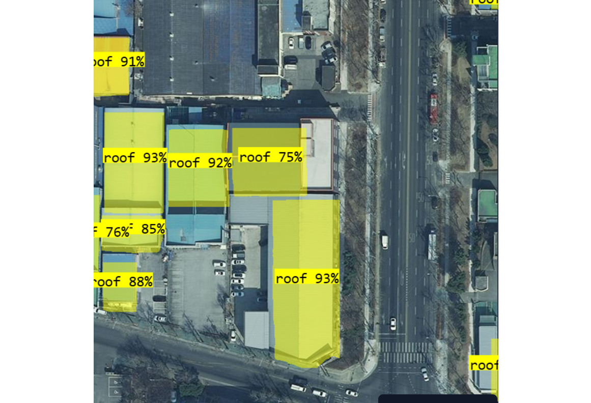
Using the coordinates from the following test image (detected by the roof detection model)
The code will generate the following output.
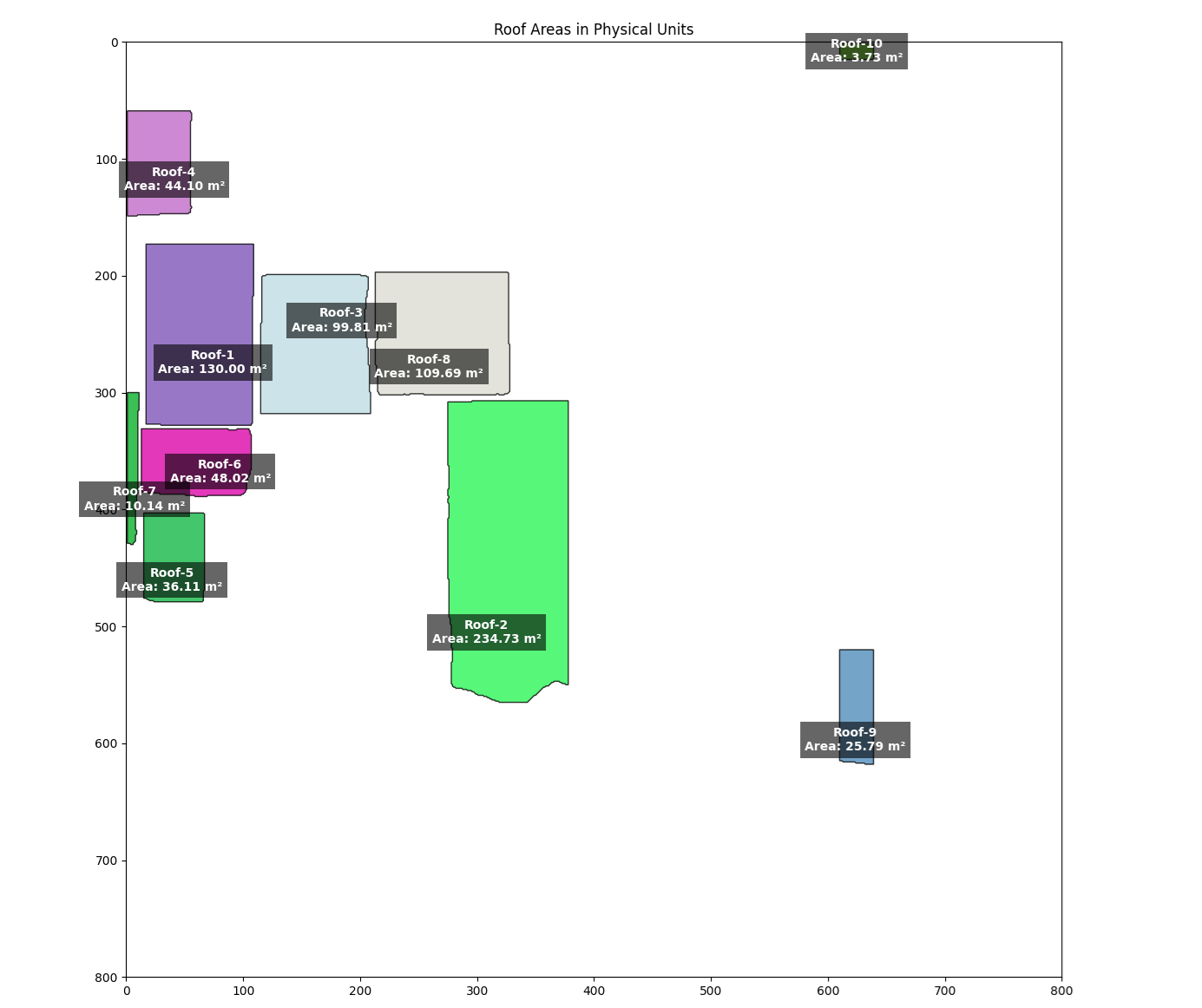
Once the roof area is calculated in square meters, it provides a foundation for estimating solar panel installations. By dividing the available roof space by the dimensions of a standard solar panel and accounting for spacing requirements, we can determine the number of panels that can be installed. This calculation enables precise planning for energy production, cost estimation, and optimal utilization of the rooftop for solar energy projects.
Conclusion
Accurately measuring rooftop areas from images is crucial for applications such as solar panel installation planning, energy optimization, and urban development. In this blog post, we demonstrated how to process model outputs, compute roof areas using the Shoelace algorithm, convert them into physical units with GSD, and visualize the results effectively.
The accuracy of rooftop measurements and physical calculations from images depend heavily on image resolution and camera parameters. High-resolution images enable precise boundary detection and minimize measurement errors, while low-resolution images may obscure details and reduce accuracy.
Camera parameters like focal length, sensor size, and capture altitude determine the GSD, which links pixel dimensions to real-world measurements.
Consistent altitude and proper camera calibration are critical to avoid distortions and inaccuracies in GSD, which directly affect the reliability of physical measurements. Accurate calibration, resolution, and capture settings are essential for applications like solar panel planning and urban development, where precise dimensions are crucial.
Cite this Post
Use the following entry to cite this post in your research:
Timothy M. (Dec 4, 2024). Solar Roof Measurement with Computer Vision. Roboflow Blog: https://blog.roboflow.com/solar-roof-measurement/
