In this blog post, you’ll learn about Simple Online and Realtime Tracking (SORT) – a real-time object tracking solution – and how to use it in your next computer vision project. We will cover some basic concepts of tracking, then go into a deep dive of how SORT works, and end with you running SORT in a Colab notebook.

Object Tracking Overview

Object tracking is a fundamental task in computer vision. It empowers object detection by following an object through time, establishing its trajectory and maintaining its identity across the frames of a video. The ability of tracking objects has a wide array of applications, ranging from player tracking in sports analytics to autonomous driving systems where understanding the movement of pedestrians, vehicles, and other objects is critical for safety and navigation.

The task of accurate real-time tracking has always been a challenging task. While researchers developed different tracking methods to address this, there is a clear need for a method that is both robust and efficient for online real-world applications. This is where Simple Online and Realtime Tracking (SORT) comes into play, proposing a simple approach to tackle the multiple object tracking problem. To use it easily, we can count the Trackers library, which has this and more trackers available for us.

What is SORT?

SORT is a method published in 2017 that took advantage of the advancements in Object Detection, which became faster and more accurate in the time of its release. When it was released, it broke all the benchmarks, becoming the fastest and most accurate. Now it has been surpassed by more complex methods, but it still remains as a strong choice in low resource computing scenarios and in certain problems where it is a natural fit. Let’s take a look at its upsides and downsides:

Pros:

• It's Super lightweight: requires little extra memory and runs on CPU.
• It's simple: only uses a combination of well-known methods, without special handling of edge cases.
• It’s really fast: in the paper (2017) it ran at 260 frames per second, while having a top accuracy. 
• It's model independent: you can use any Object Detector with it, and it hasn't a trainable model behind.

Cons:

• Doesn’t consider appearance features: matching is only based on the position and estimated trajectory of the object.
• Can’t handle objects that disappear from the scene: because of the lack of appearance features in the track, once that the object disappears from the scene, there is no mechanism to recover the track.
• Might confuse when objects overlap: when 2 trajectories are similar it might confuse because it doesn’t account for object appearance, 
• Can fail to track objects that have a big change in velocity: this is due to the linear constant velocity model used by the Kalman filter.

How does SORT work?

The main idea is simple, SORT uses a Kalman Filter for estimating how the objects are going to evolve and then these predictions are compared with the actual detected objects, in order to find where the object will be in the following timestep.

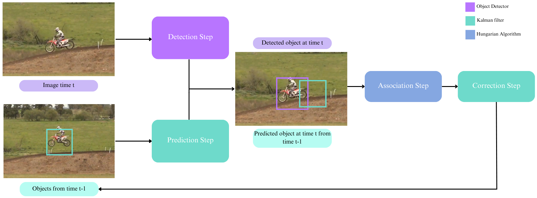
This methodology can be decomposed in the following steps:

• Detection: use an object detector to detect the bounding boxes.
• Prediction: use the Kalman Filter to predict where objects are going to move.
• Association: associate the prediction step results with the detection results.
• Correction: refine object positions with the Kalman Filter correction step.

Detection

Firstly, we need to detect the objects in the images. For this, the original paper uses Faster Region CNN (FrCNN), but it could really use any object detector like the SOTA detector RF-DETR.

After the model outputs the detected objects they only keep the objects with output probabilities greater than 50% to the tracking framework, but the trackers library lets us vary this threshold.

Prediction

So once that we have the detected objects at time t, we would like to know which of them were present at time t-1 and match them. In order to do this, authors propose to predict where the objects are going to move and then match the ones with the closest IoU between the detected at time t, and the predictions of movement of the objects at time t-1 in what we call the Association Step.

To do this prediction, they propose a linear constant velocity model, which is independent of other objects and camera motion. Then, the optimal velocity for the object is solved with a Kalman Filter.

Kalman Filters

The Kalman Filter is a method to estimate the state of a dynamic system (in our case the position of the object) where you have the equations that describe its approximated behavior and want to refine the estimated state with noisy measurements (the object detections).

Kalman Filters are optimal for linear dynamical systems, and for SORT we make the assumption that we have a linear constant velocity model. This basically consists in assuming that the velocity of the object will remain almost constant, just changing because of a noise term that the model has, and with this velocity it can predict the next position in what we call the prediction step. 

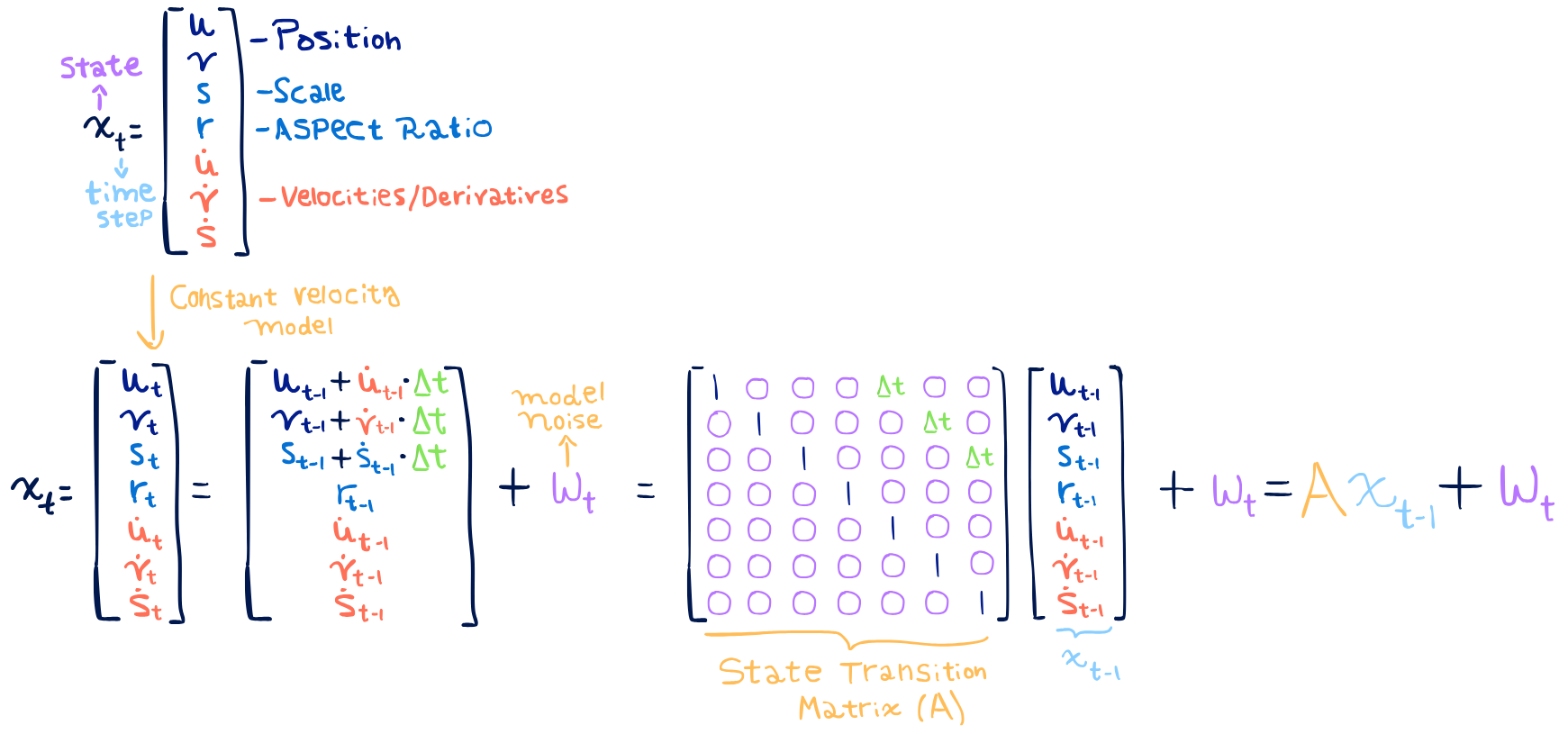
So let’s write down the model that SORT proposes for the Kalman Filter. To begin with, the state that we have at each time step will include:

• The position (u and v)
• The scale of the object and the aspect ratio of the bounding box
• The velocities in the horizontal and vertical direction and the change in the scale, which is expected to be minimal. The aspect ratio shouldn't change, so they don’t model its velocity.

Because it is a linear velocity model, using some physics knowledge we know that when travelling at a constant speed, the distance that the object will travel is the speed times the travelling time. So the state at time t can be derived from the state at time t-1, in a recurrent equation. This model looks like:

Because we are not completely certain of the state, Kalman Filters model it with a Gaussian distribution, which has 2 parameters: the Mean (μ) and Covariance(Σ). In visual terms, this can be seen in the following image, where we are tracking a motorcycle.

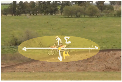
In the beginning of this process, we will have high uncertainty on the real position of the motorcycle and its speed, but with several detection we will be more and more certain. 

So, how do Kalman filters adjust the estimate?

Let’s take a look at an overview of the algorithm 

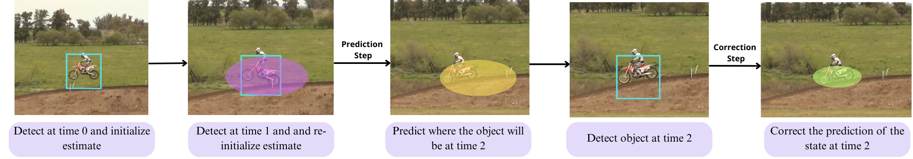
Kalman filters begin its algorithm by specifying the covariance matrices for the errors, the initial state and then it will move forward in time by doing the prediction and correction steps. The estimates at the first time steps might be noisy, but with each new detection the estimates will be refined, achieving highly accurate estimates.

Kalman Filter Prediction Step

The prediction step consists of updating our belief of the state, predicting through the transition model the expected value t-1 and the covariance matrix   t-1. Their update looks like:

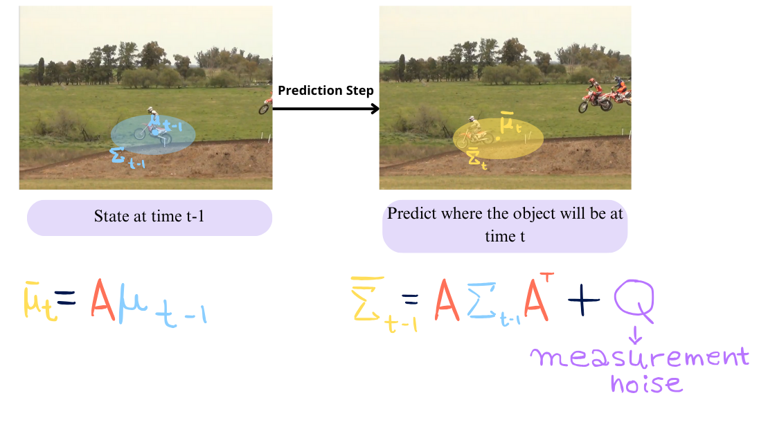
So out of this step we get where the filter thinks that the object will be based on the linear velocity model (mean) and a measure of how sure it is of the prediction (covariance).

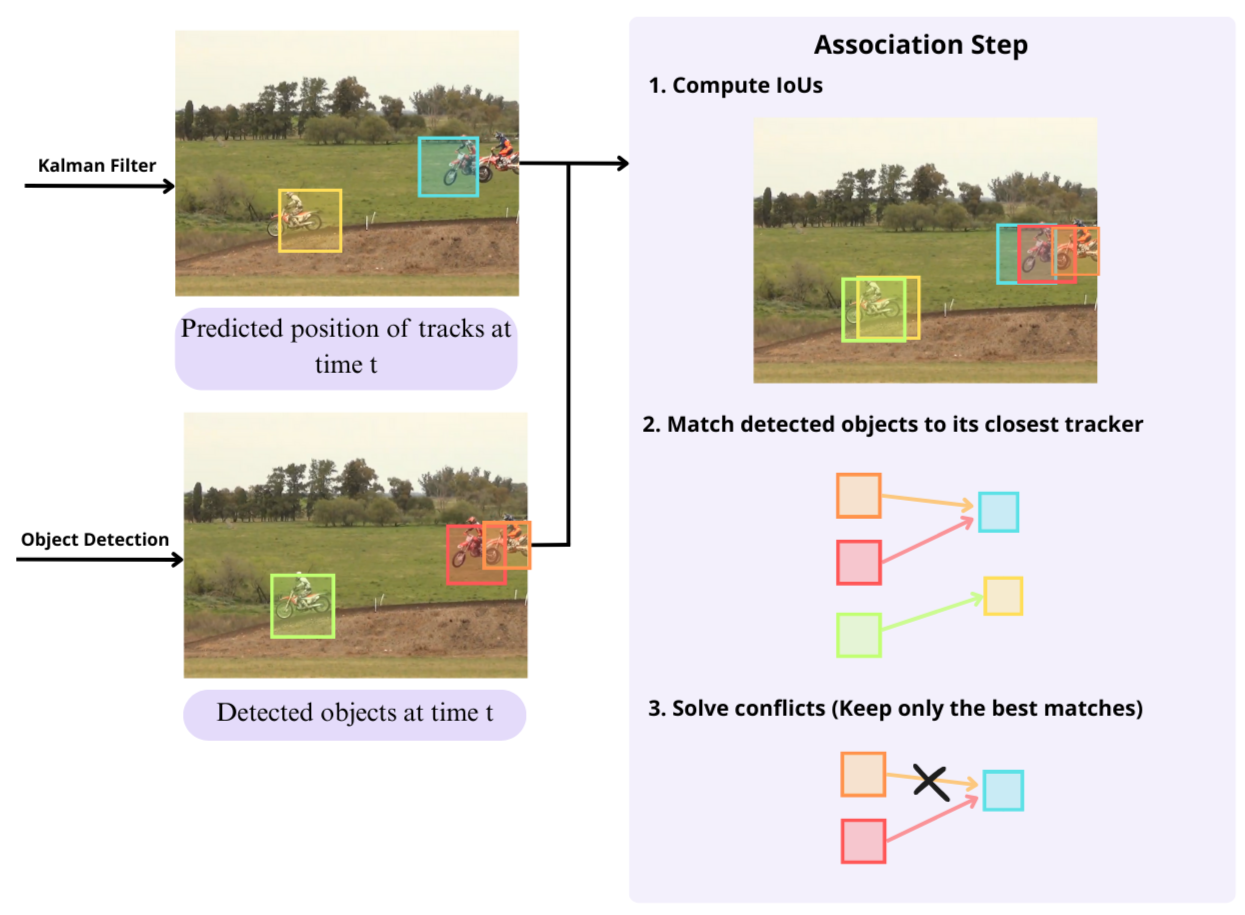
Association

In the association step, we will match the results of the prediction step and detection step, which are bounding boxes. We will match the movement predictions from time t-1 to its closest object in the time t using Intersection over Union (IoU) metric. The assignment is solved optimally using the Hungarian algorithm. Additionally, a minimum IOU is imposed to reject assignments where the overlap is small. The procedure can be visualized in the following figure.

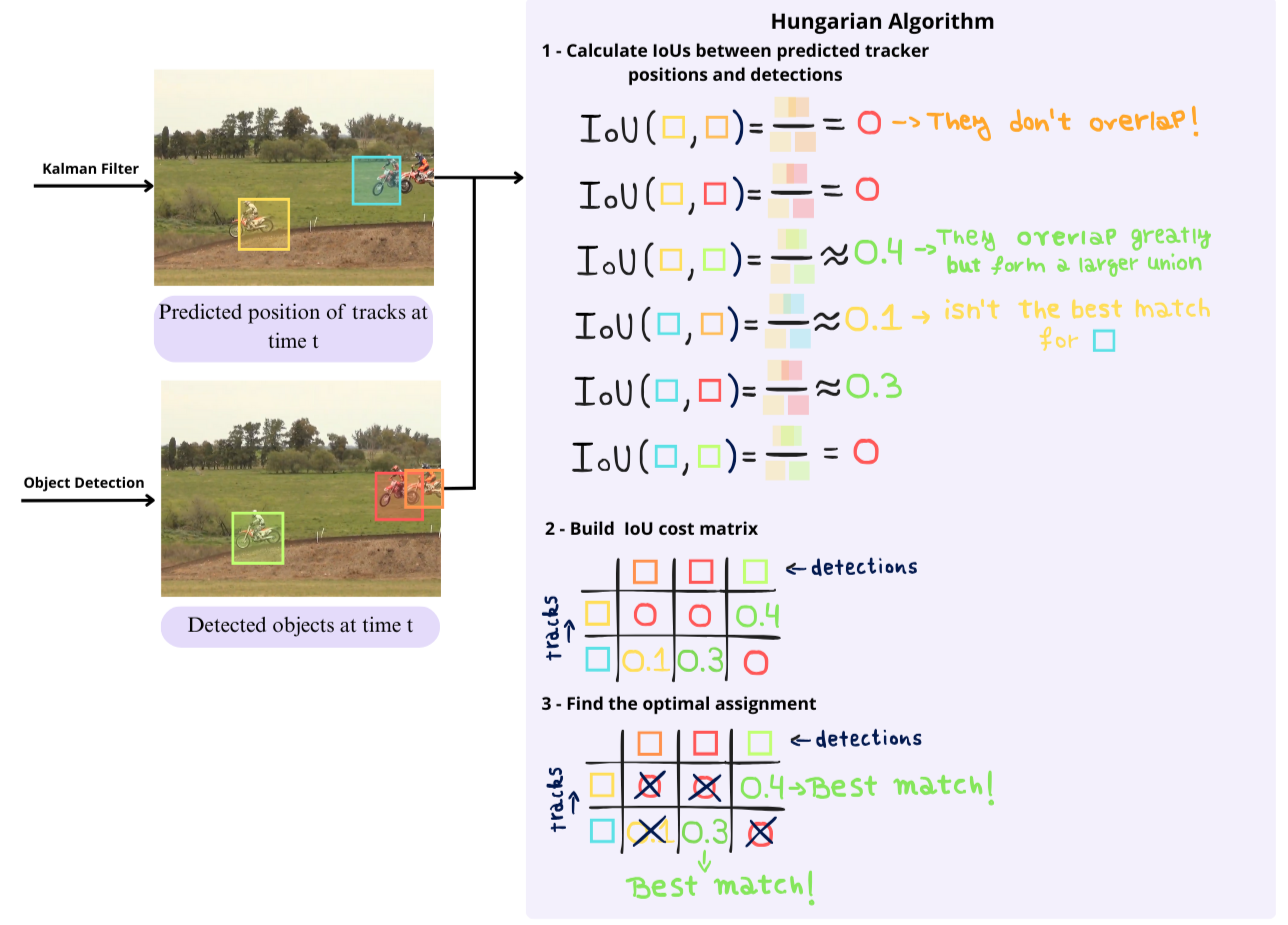
Hungarian algorithm

The problem that the Hungarian Algorithm addresses is the matching of each element with its closest in the other sequence.  The difficulty here is that from sequence 1 we might have 2 different elements such that its closest is the same in sequence 2, but only one can keep that match. We could try and brute force the solution, but in this way assigning n elements to n slots has a time complexity of O(n!), which makes it impossible to scale. 

That's where the Hungarian Algorithm comes useful, reducing the complexity to a polynomial  one of O(n3). The procedure to solve this problem can be seen in the following figure, in which we first compute the IoUs between the predicted tracks positions and the detection, put them in matrix form and keep only the ones that maximize the cost overall.

Correction

Once we make the matches, the Kalman Filter can refine our detected objects and velocity based on the velocity model that we imposed. This is just the classic Kalman Filter Correction step, where we compute the Kalman Gain and adjust the object position weighting the object detection and the linear model prediction, taking into consideration the detection and prediction noise. 

If there is a tracked object that hasn’t had a match, it will not correct it, but will keep track of it with only the prediction step.

Kalman Filter Correction Step

The correction step leverages the measurement information in order to adjust the prediction of the model. Because both our model and measurements are imperfect, we don't exactly know where our object really is, but we can try to use all the information we have in order to make the best estimation.

In order to do this, we are going to compute the Kalman Gain, which defines how much importance the measurement will have. Then, we will update our estimated state and covariance weighting the measurement by the Kalman Gain. A higher kalman gain indicates that we should pay more attention to the measurement than to the model. 

Let’s visualize this: 

The updated mean state estimate will basically move where we expected the object to be. In order to do this, we add to the predicted mean the weighted by the kalman gain difference between the measurement (detected object position) and between the predicted position

The updated covariance will reflect how certain we are of this new estimate, typically decreasing. For doing this, we subtract the predicted covariance weighted by the kalman gain to the predicted covariance itself.

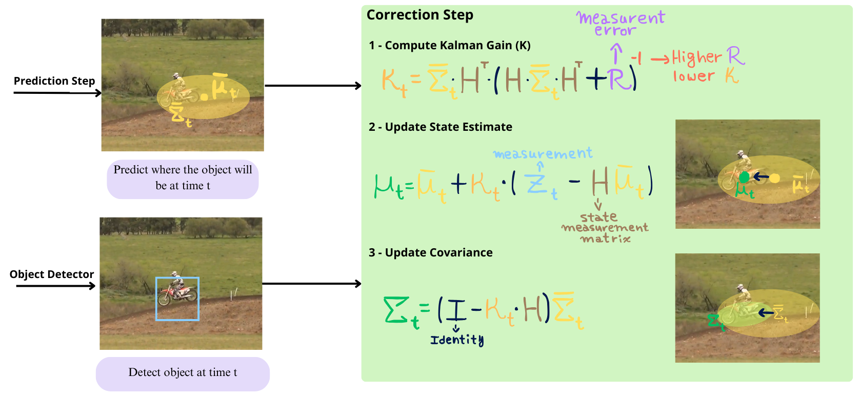
The measurement matrix H just transforms the state to the measurement space, because we don’t have sensors that measure all the state. In our case, we only measure where the object is and its size (by detecting the bounding box), so we measure everything but velocities. H will reflect this, leaving out the velocities of the measurement comparison.

And that’s it, the Kalman Filter enables us to have a comparison target for then associating the predicted state vs the detected objects, and then gives us refined object detections using the Correction Step with the detected boxes and the expected movement.

How to use SORT in Python

Luckily, the Trackers library has SORT and many other tracking methods already implemented for our usage!

Installs and setup

To begin with, we will install and import the required libraries. We will use Roboflow’s Supervision for visualization, Trackers for the SORT implementation and Yolo V8 as the object detector.

!pip install -q inference-gpu
!pip install -q trackers

Then, we will define the supervision annotators and colors for displaying the results.

import supervision as sv

color = sv.ColorPalette.from_hex([
    "#ffff00", "#ff9b00", "#ff8080", "#ff66b2", "#ff66ff", "#b266ff",
    "#9999ff", "#3399ff", "#66ffff", "#33ff99", "#66ff66", "#99ff00"
])

box_annotator = sv.BoxAnnotator(
    color=color,
    color_lookup=sv.ColorLookup.TRACK)

trace_annotator = sv.TraceAnnotator(
    color=color,
    color_lookup=sv.ColorLookup.TRACK,
    thickness=2,
    trace_length=100)

label_annotator = sv.LabelAnnotator(
    color=color,
    color_lookup=sv.ColorLookup.TRACK,
    text_color=sv.Color.BLACK,
    text_scale=0.8)

Object Tracking

We will now define our tracker and then define the tracking pipeline in the callback function.

First we will initialize a default SORT tracker which will start tracking objects if detected 3 or more times and with a minimum IoU threshold of 0.3.

from trackers import SORTTracker
tracker = SORTTracker()

Secondly, we will load our object detector, in this case we use yolov8, which we will load using the inference library.

from inference import get_model
model = get_model("yolov8m-640")

Now lets define the callback function, which will tell for each frame how to execute the object tracking.

CONFIDENCE_THRESHOLD = 0.3 # Which bounding boxes to keep from the detector
NMS_THRESHOLD = 0.3

SOURCE_VIDEO_PATH = "/content/bikes-1280x720-1.mp4"
TARGET_VIDEO_PATH = "/content/bikes-1280x720-1-result.mp4"

frame_samples = []

def callback(frame, i):
    result = model.infer(frame, confidence=CONFIDENCE_THRESHOLD)[0]
    detections = sv.Detections.from_inference(result).with_nms(threshold=NMS_THRESHOLD)
    detections = tracker.update(detections)

    annotated_image = frame.copy()
    annotated_image = box_annotator.annotate(annotated_image, detections)
    annotated_image = trace_annotator.annotate(annotated_image, detections)
    annotated_image = label_annotator.annotate(annotated_image, detections, detections.tracker_id)

    if i % 30 == 0 and i != 0:
        frame_samples.append(annotated_image)

    return annotated_image

And then we can proceed to run the object tracking and visualize the final results with:

tracker.reset()

sv.process_video(
    source_path=SOURCE_VIDEO_PATH,
    target_path=TARGET_VIDEO_PATH,
    callback=callback,
    show_progress=True,
)
sv.plot_images_grid(images=frame_samples[:4], grid_size=(2, 2))

So the final result that we get of doing this is:

Conclusion

In this blog we explored how the SORT tracker works, learning in detail how it’s able to efficiently track objects, we learned about its advantages and limitations and finally we used the brand new Trackers library to easily use this tracker with Python.

Cite this Post

Use the following entry to cite this post in your research:

Alexander Dylan Bodner. (May 27, 2025). SORT Explained: Real-Time Object Tracking in Python. Roboflow Blog: https://blog.roboflow.com/sort-explained-real-time-object-tracking-in-python/