
OpenAI's CLIP model can auto-label image classification datasets by computing cosine similarity between image embeddings and text embeddings for each class name, then assigning the best-matching label. This tutorial walks through the full pipeline in a Jupyter notebook using the Roboflow Art Classification Dataset, covering installation, feature extraction, similarity scoring, and writing results to a CSV ready for upload to Roboflow.
Labeling large datasets can be a time-consuming and labor-intensive task. However, with advancements in deep learning and natural language processing, it is now possible to automate the labeling process.
In this blog post, we will guide you through the process of using CLIP (Contrastive Language-Image Pretraining) and Roboflow to automatically label your dataset directly within a Jupyter Notebook environment.
What is CLIP?
CLIP, developed by OpenAI, is a cutting-edge deep learning model designed to extract visual concepts from natural language descriptions. This model achieves cross-modal retrieval and understanding by associating images and text within a shared embedding space. Through extensive training on large corpora of images and their corresponding textual descriptions, CLIP learns to encode images and text in a way that their embeddings reflect semantic similarity.
Automatically Labeling Classification Datasets
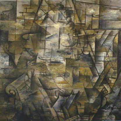
For this demonstration, we will be using the Roboflow Art Classification Dataset. This classification dataset contains artistic movement art images that range from Abstract Expressionism to Pop Art. The dataset has been curated and labeled to include a diverse range of artistic styles, allowing us to explore the capabilities of CLIP and automated labeling.
Step 1: Installation and Setup
Before we dive into autolabeling, let's set up the required environment. We'll be using a Jupyter notebook for this demonstration. Start by installing the necessary dependencies:
!pip install ftfy regex tqdm
!pip install git+https://github.com/openai/CLIP.git
!pip install roboflow
Next, import the required libraries:
import glob
import os
import clip
import math
import torch
import matplotlib.pyplot as plt
from IPython.core.display import HTML
import numpy as np
from PIL import Image
from roboflow import Roboflow
import csv
Step 2: Loading the Dataset
Next, we need to prepare our dataset for autolabeling. If you don't have a Roboflow account, you can sign up for free and create a new project.
Once you have your project set up on Roboflow, you can use the Roboflow Python package to download the dataset directly into your Jupyter notebook. Here's an example of how to download the dataset:
rf = Roboflow(api_key="YOUR_API_KEY")
project = rf.workspace("art-dataset").project("wiki-art")
dataset = project.version(2).download("clip")
Step 3: Extracting Image Features
To automatically label the dataset, we need to extract features from the images using the CLIP model. Execute the following code to extract the image features:
for i in range(batches):
 images = img[i*batch : (i+1)*batch]
 batch_preprocessed = batch_preprocessed = torch.stack([preprocess(i) for i in images if i is not None]).to(device)

 with torch.no_grad():
   image_embeddings = model.encode_image(batch_preprocessed)
   image_embeddings /= image_embeddings.norm(dim=-1, keepdim=True)

 features = torch.cat((features, image_embeddings))

print(f"Images Extracted: {features.shape}")
Step 4: Finding Similar Images with Text Input
Now, let's use the extracted image features to find similar images based on a text input. Execute the following code to define a function that finds similar images given a text query:
def findImg(input_text, threshold=25.9, num=5):
 with torch.no_grad():
   text_embeddings = model.encode_text(clip.tokenize(input_text).to(device))
   text_embeddings /= text_embeddings.norm(dim=-1, keepdim=True)

 similarities = (100.0 * features @ text_embeddings.T)
 values, top_poster = similarities.topk(num, dim=0)

 for frame_id in top_poster:
   score = similarities[frame_id.item()]
   if score > threshold:
     print("Cosine Similarity Score for Image", frame_id.item(), ":", score)
     display(img[frame_id])

findImg("Cubism")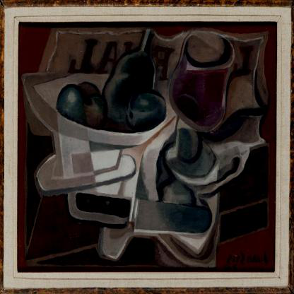
This function takes an input text and finds the most similar images based on the cosine similarity between the text and image embeddings. You can adjust the threshold parameter to control the similarity threshold for displaying images. Replace the text query with your own description to find relevant images.
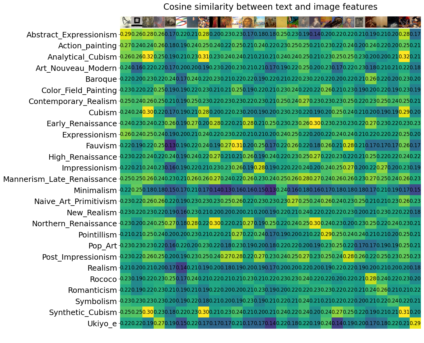
Step 5: Visualizing Cosine Similarity between Text and Image Features
To visualize the similarity between the text and image features, you can refer to the complete code provided in the interactive notebook.
We compute the cosine similarity between the text and image features and visualize it as a heat map. Each row represents a text description, and each column represents an image class. The values in the heatmap indicate the similarity scores between the text and image features.
Step 6: Autolabeling with CLIP
Finally, let's perform automatic labeling of the dataset using the CLIP model. Execute the following code:
class_tokens = clip.tokenize([desc for desc in labels]).cuda()
with torch.no_grad():
   text_features = model.encode_text(class_tokens).float()
text_features /= text_features.norm(dim=-1, keepdim=True)
img = []
features = torch.empty([0, 512], dtype=torch.float16).to(device)

header = ["Names"] + labels
rows = []

for i in range(0, len(image_paths), batch):
   batch_paths = image_paths[i : i + batch]

   for path in batch_paths:
       img_name = os.path.basename(path)
       with Image.open(path) as im:
           im_array = np.array(im)
           new_im = Image.fromarray(im_array)
           img.append(new_im)

   images = img[-len(batch_paths):]
   batch_preprocessed = torch.stack([preprocess(i) for i in images if i is not None]).to(device)

   with torch.no_grad():
       image_embeddings = model.encode_image(batch_preprocessed)
       image_embeddings /= image_embeddings.norm(dim=-1, keepdim=True)

   features = torch.cat((features, image_embeddings))

   similarity_scores = np.dot(image_embeddings.cpu().numpy(), text_features.cpu().numpy().T)
   most_similar_labels = np.argmax(similarity_scores, axis=1)

   for img_name, label in zip(batch_paths, most_similar_labels):
       row = [os.path.basename(img_name)]
       for j in range(len(labels)):
           if label == j:
               row.append(1)  # Most similar label, assign 1
           else:
               row.append(0)  # Other labels, assign 0
       rows.append(row)

filename = "autolabel.csv"  # Replace with your desired file name
with open(filename, "w", newline="") as file:
   writer = csv.writer(file)
   writer.writerow(header)
   writer.writerows(rows)
This code performs automatic labeling by calculating the cosine similarity between the image features and class text embeddings. To provide a visual representation of the process, consider the following image which illustrates the underlying concept:
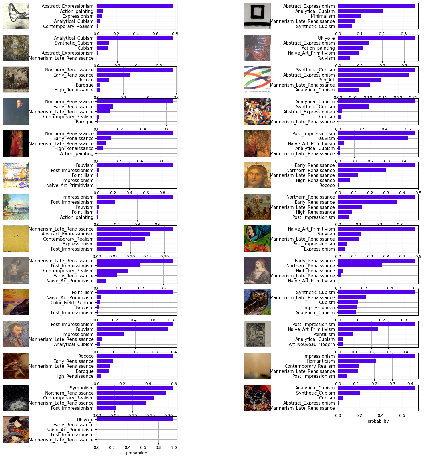
The labels are then saved in a CSV file named "autolabel.csv".
Conclusion
You have successfully automated dataset labeling using CLIP and Roboflow within a Jupyter Notebook. This process can significantly save time and effort in labeling large datasets! Happy Engineering!
Cite this Post
Use the following entry to cite this post in your research:
Arty Ariuntuya. (Jun 7, 2023). Auto-Label Classification Datasets Using CLIP. Roboflow Blog: https://blog.roboflow.com/how-to-auto-label-classification-datasets/