
Released on October 2nd, 2025, RF-DETR Segmentation is a state-of-the-art instance segmentation model. You can use this model architecture to identify, with pixel-precision, the location of objects in an image.
RF-DETR is accompanied by a paper, RF-DETR: Neural Architecture Search for Real-Time Detection Transformers, which is available on Arxiv. The paper contains detailed information about the RF-DETR model architecture, our results from benchmarking the model, and more.
In this guide, we are going to walk through how to train an RF-DETR Segmentation model using the rfdetr Python package. We will then deploy our model to the cloud.
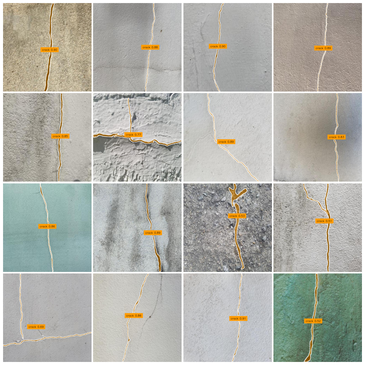
We will train a model that can identify cracks in concrete. Here is an example of results returned by the model we will train:
Without further ado, let’s get started!
You can follow along with this guide using our Colab training notebook. We recommend training with an A100 GPU.
Step #1: Dataset Preparation
Before we train a model, we need to prepare a dataset in the Microsoft COCO JSON Segmentation format. For this guide, we are going to use a dataset of concrete cracks available on Roboflow Universe, the largest community of annotated computer vision datasets and models on the web.
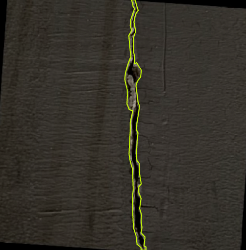
Here is an example of an image from the dataset, showing a crack:
You can follow along with this guide using any dataset you want, although you will need a dataset in the COCO JSON Segmentation format for use with training an RF-DETR model.
If you need to convert a dataset to COCO JSON Segmentation, you can upload it to Roboflow and export the data in the COCO JSON Segmentation format.
If you need to label a dataset, you can do so using Roboflow Annotate, our fully-featured, web-based annotation tool. Annotate comes with a range of tools to speed up the labeling process, including a suite of AI-assisted labeling tools.
Step #2: Install Dependencies and Configure Environment
With a dataset ready, we can start training a model.
To get started, first install the rfdetr Python package:
pip install rfdetrNext, run !nvidia-smi in your training notebook to make sure you have an NVIDIA GPU available:
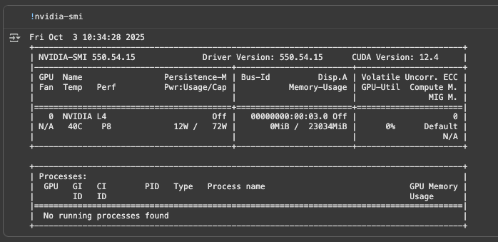
We recommend training RF-DETR models with an A100 GPU.
Step #3: Download a Dataset
We need to download our dataset into our notebook for use in training. We can do this using the Roboflow Python package.
First, set your Roboflow API key in an environment variable called ROBOFLOW_API_KEY. Learn how to retrieve your Roboflow API key.
Then, run the following code:
from roboflow import download_dataset
dataset = download_dataset("https://universe.roboflow.com/roboflow-jvuqo/creacks-eapny/4", "coco")
If you have a private dataset on Roboflow that you want to download for use in training, open a version of your dataset in Roboflow, then click the “Download Dataset” button. You will then be able to choose to export your data in the COCO Segmentation format.
Step #4: Start Training
We are now ready to train our model.
For this guide, we are going to use the RFDETRSegPreview trainer. Run the following code to start a training job:
from rfdetr import RFDETRSegPreview

model = RFDETRSegPreview()

model.train(dataset_dir=dataset.location, epochs=5, batch_size=4, grad_accum_steps=4)
Choosing Epochs
For this example, we are training for 5 epochs. Since DETR models tend to stabilize in fewer epochs than YOLO models, this will be enough to help us see how well RF-DETR performs on our dataset. With that said, for a production model, we would recommend training for at least 50 epochs. This will ensure you train for long enough for your model to achieve the best performance.
Choosing Batch Size
Different GPUs have different amounts of VRAM (video memory), which limits how much data they can handle at once during training. To make training work well on any machine, you can adjust two settings: batch_size and grad_accum_steps.
These control how many samples are processed at a time. The key is to keep their product equal to 16 — that’s our recommended total batch size. For example, on powerful GPUs like the A100, set batch_size=16 and grad_accum_steps=1.
On smaller GPUs like the T4, use batch_size=4 and grad_accum_steps=4. We use a method called gradient accumulation, which lets the model simulate training with a larger batch size by gradually collecting updates before adjusting the weights.
Model Configuration Options
There are several configuration options available to customise your training job. For example, you can log training metrics with Tensorboard, configure early stopping, and more. To learn about all of the arguments the train() function accepts, refer to the RF-DETR training documentation.
Once you have trained your model, you can visualize the model metrics with the following code:
from PIL import Image
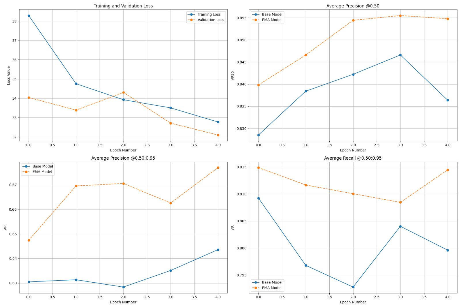
Image.open("/content/output/metrics_plot.png")Loss should decrease over time.
Here are graphs from our concrete crack detection training run showing training and validation loss and Average Precision @ 0.50, Average Precision @ 0.50:0.95, and Average Recall @ 0.50:0.95:
Clear Memory
Before benchmarking the model, we need to load the best saved checkpoint. To ensure it fits on the GPU, we first need to free up GPU memory. This involves deleting any remaining references to previously used objects, triggering Python’s garbage collector, and clearing the CUDA memory cache.
Follow our notebook to see the code you need to clear memory so you can load your trained model.
Test Your RF-DETR Segmentation Model
Once you have trained your model, you can start using it with the rfdetr Python package.
Let’s run our model on a few images from our dataset test set to see how well it performs. We will use the open source supervision Python package to choose images at random from our dataset test set. We will also use the annotation suite in supervision to plot the masks returned by our model.
First, let’s load our dataset test set:
import supervision as sv

ds_test = sv.DetectionDataset.from_coco(
    images_directory_path=f"{dataset.location}/test",
    annotations_path=f"{dataset.location}/test/_annotations.coco.json",
    force_masks=True
)
Next, let’s load a random image from our test set and compare the ground truth to the results from our model:
import supervision as sv
from PIL import Image

def annotate(image: Image.Image, detections: sv.Detections, classes: dict[int, str]) -> Image.Image:
    color = sv.ColorPalette.from_hex([
        "#ffff00", "#ff9b00", "#ff8080", "#ff66b2", "#ff66ff", "#b266ff",
        "#9999ff", "#3399ff", "#66ffff", "#33ff99", "#66ff66", "#99ff00"
    ])
    text_scale = sv.calculate_optimal_text_scale(resolution_wh=image.size)

    mask_annotator = sv.MaskAnnotator(color=color)
    polygon_annotator = sv.PolygonAnnotator(color=sv.Color.WHITE)
    label_annotator = sv.LabelAnnotator(
        color=color,
        text_color=sv.Color.BLACK,
        text_scale=text_scale,
        text_position=sv.Position.CENTER_OF_MASS
    )

    labels = [
        f"{classes.get(class_id, 'unknown')} {confidence:.2f}"
        for class_id, confidence in zip(detections.class_id, detections.confidence)
    ]

    out = image.copy()
    out = mask_annotator.annotate(out, detections)
    out = polygon_annotator.annotate(out, detections)
    out = label_annotator.annotate(out, detections, labels)
    out.thumbnail((1000, 1000))
    return out

model = RFDETRSegPreview(pretrain_weights="/content/output/checkpoint_best_total.pth")
model.optimize_for_inference()

import random
import matplotlib.pyplot as plt

N = 16
L = len(ds_test)

annotated_images = []

for i in random.sample(range(L), N):
    path, _, annotations = ds[i]
    image = Image.open(path)
    detections = model.predict(image, threshold=0.5)
    annotated_image = annotate(image, detections, classes={i: class_name for i, class_name in enumerate(ds_test.classes)})
    annotated_images.append(annotated_image)

fig, axes = plt.subplots(4, 4, figsize=(12, 12))

for ax, img in zip(axes.flat, annotated_images):
    ax.imshow(img)
    ax.axis("off")

plt.subplots_adjust(wspace=0.02, hspace=0.02, left=0.01, right=0.99, top=0.99, bottom=0.01)

plt.show()
Above, we define a function to visualize predictions from a model, load our model, load random images, run inference with our fine-tuned model, then plot the results.
Here are the results:
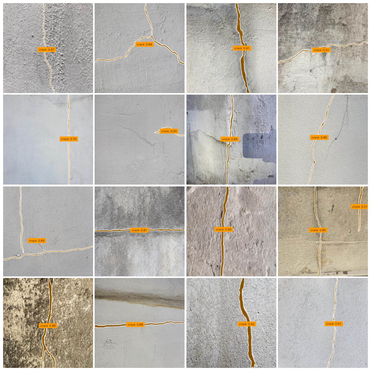
From the model inference results, we can see RF-DETR successfully identified the most prominent cracks in the images.
Deploy Your RF-DETR Segmentation Model
With a model ready, the next question is: how do I deploy it to production?
You can upload your RF-DETR model weights to Roboflow to build an application using your model with Roboflow Workflows. Workflows lets you use models with 100+ “blocks” to build multi-step computer vision applications.
For example, with Workflows you can:
- Track objects identified by a detection or segmentation model using ByteTracker, an object tracking algorithm.
- Visualise predictions from your model.
- Filter predictions.
- Crop regions identified by your model.
- Send SMS messages when a model prediction is returned.
- And more.
To learn how to get started, check out the Roboflow Workflows documentation.
Let’s set up a Workflow that runs our model and plots the predictions from our model as an example. Our Workflow will be available as a serverless cloud API that we can call, and ready for use on our own hardware too.
First, create a project in Roboflow and upload the dataset you used to train your model. This will allow you to manage all of your data within the Roboflow web application, and associate the model weights that you have trained with the dataset you used to train them.
Once you have uploaded your dataset, click "Versions" in the left sidebar and create a dataset version.
Next, we need to upload our model to Roboflow:
from rfdetr import RFDETRSegPreview

x = RFDETRSegPreview(pretrain_weights="<path/to/pretrain/weights/dir>")
x.deploy_to_roboflow(
  workspace="<your-workspace>",
  project_id="<your-project-id>",
  version=1,
  api_key="<YOUR_API_KEY>"
)
Above, set your Roboflow workspace ID, project ID, and API Key:
Set the version ID to the ID of the dataset version with which you want to associate your model weights.
Once you upload your model weights, they will then be ready for use in Workflows and deployment on-device using Roboflow Inference, an open source computer vision inference server.
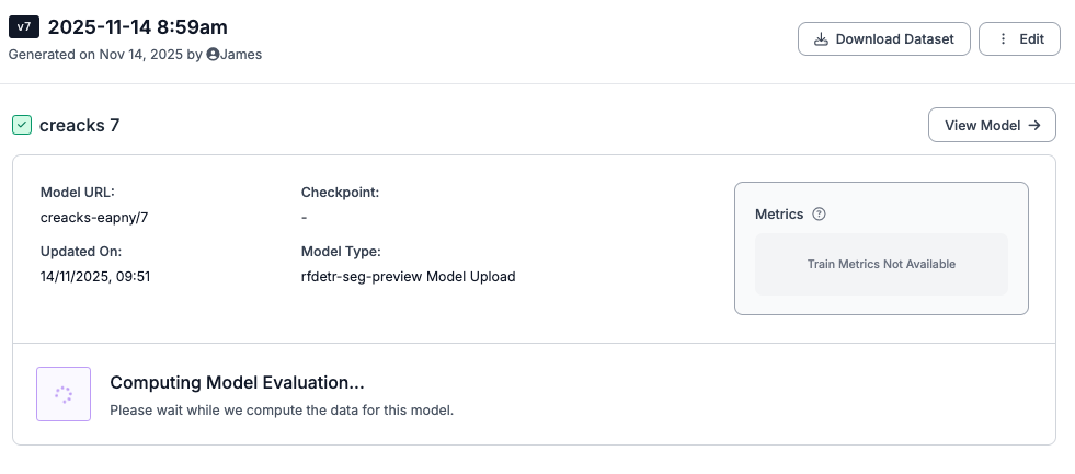
You will be able to see your model in your models list in Roboflow, too:
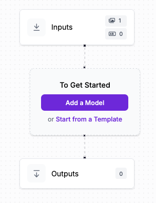
To use your model in a Workflow, click Workflows in the left sidebar of the Roboflow web application, then create a new Workflow. Then, click “Add a Model”:
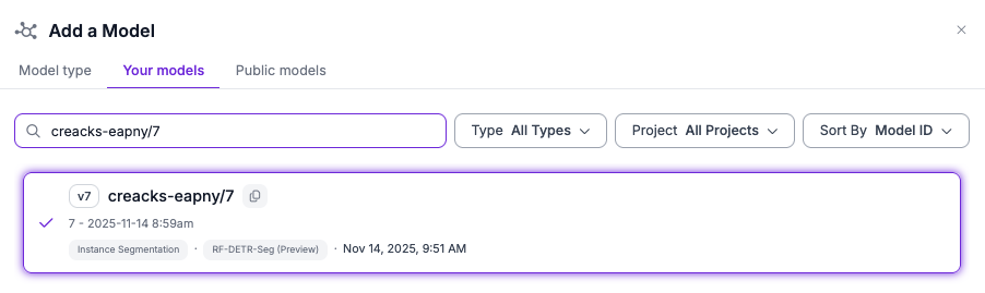
Choose the ID of the model you just uploaded:
Then, add a Mask Visualization and Label Visualization block to your Workflow. These blocks will let us visualise the predictions from our model. Your Workflow should look like this:
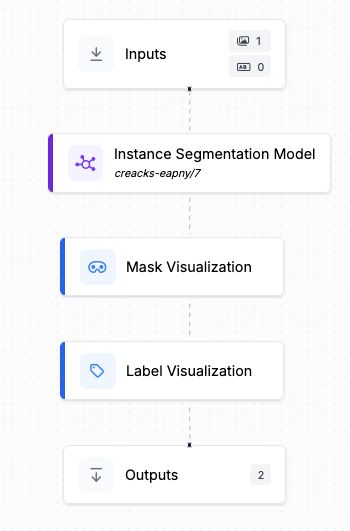
We now have a Workflow that can run our RF-DETR Segmentation model and display the results from the model on an input image.
Let’s test our Workflow.
To test your Workflow, click “Test Workflow” in the top right corner of the Workflows editor.
You can then upload an image to test your Workflow.
Here is the result from an example image:
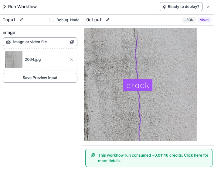
Our model successfully identifies both the crack in the concrete.
All Workflows have a serverless hosted API you can call. You can also deploy your Workflow on your own hardware. To see deployment options for your Workflow, click “Deploy” in the Workflows editor.
Conclusion
Released in October 2025, RF-DETR Segmentation is a new, state-of-the-art image segmentation model. This is the first Segmentation model in the RF-DETR family. We hope to launch three more model sizes by the end of the year.
In this guide, we walked through how to train an RF-DETR Segmentation model in Google Colab. We trained a model to identify cracks in concrete. We then uploaded our model to Roboflow. We built an application that runs our model and visualises predictions from our model using Roboflow Workflows. Our Workflow is ready to deploy in the cloud or on our own hardware
To learn more about RF-DETR, check out the RF-DETR GitHub repository.
Cite this Post
Use the following entry to cite this post in your research:
James Gallagher, Piotr Skalski. (Nov 14, 2025). How to Train an RF-DETR Segmentation Model with a Custom Dataset. Roboflow Blog: https://blog.roboflow.com/train-rf-detr-segmentation/