Vector Analysis with Scikit-learn and Bokeh

This post is part of Dataset Day in Roboflow Launch Week 2023, the day during which we have announced many new additions to our data management and annotation solutions. To see all of the announcements from launch week, check out the Roboflow Launch Week page.

Vector embeddings have become a hot topic in machine learning these days. Roboflow uses multimodal CLIP embeddings embeddings to power our dataset search feature. And, now, you can access your dataset's CLIP embeddings via the Roboflow API.

In this tutorial, we will load embeddings for a dataset from Roboflow, analyze them with the t-SNE algorithm using Scikit-learn and visualize them in an interactive plot using Bokeh.

Loading CLIP Vectors from Roboflow

Roboflow's new Search API exposes our UI's powerful dataset search feature for programmatic access. Not only can you search semantically, by class, split, and tag, but you can also retrieve the CLIP vectors for the images in your project.

Access to CLIP lets you do powerful things like image similarity search, clustering, and anomaly detection. In this tutorial, we'll be visualizing our CLIP clusters to try to find labeling errors and unexpected images in our dataset.

By default the notebook loads 1500 images' data by performing a search in a loop (loading the maximum of 250 at a time):

response = requests.post(
        search_url,
        json={
            'prompt': closest_to_text,
            'limit': 250,
            'offset': offset,
            'fields': ['id', 'owner', 'name', 'split', 'annotations', 'embedding']
        },
        headers={
            'Authorization': f'Bearer {roboflow.load_roboflow_api_key()}'
        }
    )

At the end of this process, we have an images array containing all of our search responses, including the CLIP vectors we're interested in visualizing.

t-SNE with sklearn

Next, we need reduse our 768-dimension CLIP vectors down to something more manageable that we can display on screen. We use the t-SNE algorithm to give each vector a point in 2-dimensional space while maintaining their approximate relative distances from each other. This puts "similar" images near each other.

tsne = TSNE(n_components=2, verbose=1)
z = tsne.fit_transform(np.array([image['embedding'] for image in filtered_images]))

This algorithm is iterative and can take a minute or two to finish depending on the size of your dataset.

Visualizing with Bokeh

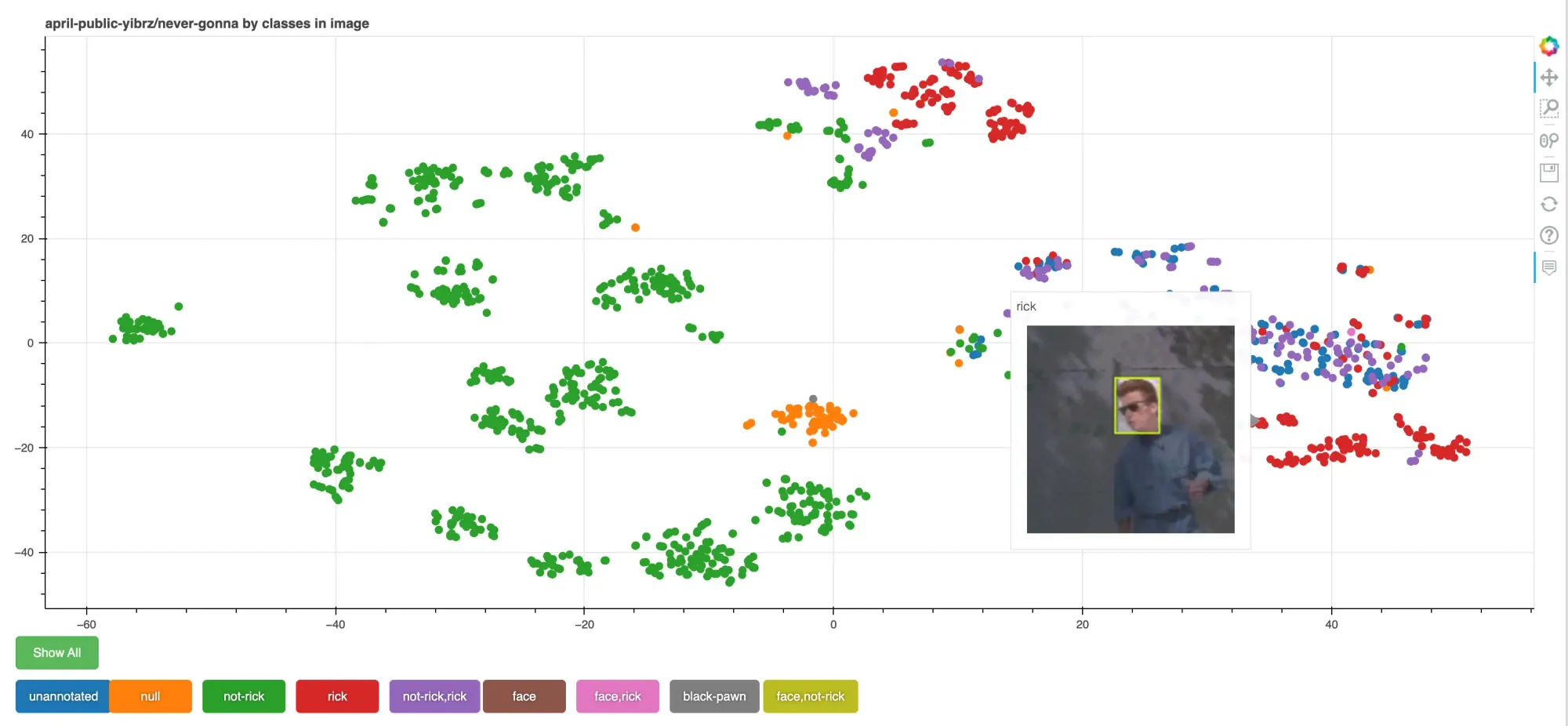
Now we'll create an interactive visualization using a library called Bokeh. First, we give each data point a class (and we'll use this to color the points in our plog). There are 3 options built into the script, but you can customize it to visualize whatever features of your dataset you like.

• classes in image visualizes the different types of objects of interest the dataset contains. You should expect the colors to be clustered near each other because they should be semantically similar. If you see outliers, it might signify labeling error or interesting edge cases to look at.
• object count shows the number of objects labeled in each image. This can be useful for looking at the distribution. For instance, images with zero labeled objects might be a sign that you missed something when labeling.
• train/valid/test split shows how similar your training and testing data are. If they're very disjoint it might signal that your metrics are not measuring what you think they are and your model might struggle in the wild.

You can use the buttons below the chart to filter which clusters are shown.

Next Steps

The notebook is setup to analyze any Roboflow dataset. Use it to explore your data and see if you can find any interesting anomalies or outliers.

You can adapt and customize this script to your own needs using our search API and metadata like tags you've applied to your images in Roboflow to discover other insights that will help you improve your models.

If you find something neat, let us know on the forum!

Cite this Post

Use the following entry to cite this post in your research:

Brad Dwyer. (Mar 29, 2023). Vector Analysis with Scikit-learn and Bokeh. Roboflow Blog: https://blog.roboflow.com/vector-analysis/

Discuss this Post

If you have any questions about this blog post, start a discussion on the Roboflow Forum.