Visual Anomaly Detection

In production environments, your biggest threat isn't the defect you’ve seen a thousand times: it’s the unusual patterns you've never seen before. Visual anomaly detection solves this by teaching a system what “normal” looks like, and then identifying anything that does not fit that pattern. Today we'll do a deep dive into catching these unknown knowns with anomaly detection, and share how to build a practical anomaly detection workflow with Roboflow.

What Is Visual Anomaly Detection?

Visual anomaly detection is a computer vision technique where a model learns the normal appearance of objects or scenes, and then detects anything that significantly deviates from that normal pattern. In short, it answers: “Does any part of this image look unusual compared to normal examples?”

Modern visual anomaly detection systems typically produce an anomaly score to show how abnormal an image is, and an anomaly map or heatmap to show where the unusual region is located.

Defining “Normal” (Data Acquisition)

The success of a visual anomaly detection system depends on how well it learns what normal looks like. In anomaly detection research, normal data means the set of samples the system is supposed to treat as valid, expected, and non-anomalous for the task.

This means data acquisition is not just about collecting many images, but about collecting the right normal images. The dataset should capture the true variation of good products under real operating conditions, including small differences in texture, lighting, position, orientation, and surface appearance. If these normal variations are missing from the training data, the model may wrongly flag them as anomalies later.

In practice, defining normal starts with capturing images from the same camera setup and environment that will be used during deployment. The background, lighting, distance, angle, and product placement should be as consistent as possible, because visual anomaly detection is highly sensitive to changes that are not actually defects. It is also important to collect normal samples across different batches, times, and operating conditions so the model learns realistic normal variation instead of a narrow, overly perfect version of it.

The definition of normal is always task specific. In many industrial anomaly detection settings, normal data is made up of defect-free or anomaly-free samples. That is how widely used benchmarks are constructed. MVTec AD uses defect-free images for training, while anomalous samples appear at test time. MVTec 3D-AD and MVTec AD 2 follow the same pattern with defect-free training and validation sets. This is why, in factory inspection, “normal” often looks very close to “good.”

But research does not limit normal to a single perfect class. In anomaly detection, normal data can also include multiple valid classes, as long as those classes belong to the intended inlier distribution. The key question is not “Is this sample perfect?” but “Is this sample part of the valid data distribution the model was meant to accept?”

Normal can refer not only to visually defect-free surfaces, but also to compositionally valid scenes. In datasets such as MVTec LOCO AD, the training images are anomaly-free, yet anomalies in the test set may arise from invalid object counts, placements, or combinations rather than surface defects alone. In this context, normality requires that both the individual components and their spatial or logical relationships are correct.

Conceptually this is a fascinating shift in machine vision. Classical inspection asks whether an object is damaged. LOCO AD asks whether a configuration makes sense. That difference nudges anomaly detection toward something closer to structured reasoning, which is why many recent papers treat LOCO AD as a bridge between industrial inspection and higher-level scene understanding.

The goal is to teach the system that normal does not mean one exact image. Normal is a range of acceptable appearances. A good dataset should therefore include clean examples of products that are all acceptable, even if they show slight natural differences. Once this normal baseline is learned, the model can compare new images against it and identify regions that fall outside that expected range.

Types of Visual Anomalies

Not all anomalies are the same. The type of anomaly you face determines which method to use. The research community and standard benchmarks distinguish between several categories.

Structural anomalies: Structural anomalies are physical defects that change the surface or shape of an object. Examples include scratches, dents, cracks, holes, contamination, stains, or chips. These anomalies are usually local, affecting only a small region of the image.

Logical anomalies: Logical anomalies occur when the arrangement of components is incorrect, even though each component appears visually normal. Examples include a missing cable, wrong component placement, incorrect ordering, or an extra object. These anomalies are harder to detect because the problem lies in the relationship between components, not surface defects.

Textural anomalies: Textural anomalies involve subtle deviations in surface patterns or materials, such as irregular fabric weave, wood grain variation, coating inconsistencies, or color shifts. These are difficult to detect because the difference from normal texture may be very small.

Semantic or scene-level anomalies: Semantic or scene-level anomalies occur when the entire scene contains something unexpected, such as the wrong product on a line, a person in a restricted area, or a foreign object in view.

Hierarchical Anomalies and Patch vs. Entity Level: Anomalies can also appear at different levels of granularity. Patch-level anomalies affect small regions of an image, such as scratches or bent pins. Entity-level anomalies involve entire objects that do not belong, such as a wrong product on a conveyor.

In practice, many real-world systems encounter a mix of these anomaly types. This is why modern inspection pipelines often combine local patch analysis with global reasoning methods.

The Main Methods of Anomaly Detection

Visual anomaly detection is not a single technique, but a broad family of approaches. The following list combines learning strategies, model families, and data settings commonly used in visual anomaly detection.

1. Fully Supervised

In the fully supervised setting, both normal and defective samples are annotated. Depending on the task, these annotations may be image-level labels, bounding boxes, or pixel-level masks. This setting provides the richest semantic information about known defects, and usually gives the best accuracy when defect types are known, stable, and well represented in the training data. The tradeoff is that annotation cost is the highest, and generalization to new, unseen defect types is limited.

In industrial inspection, models such RF-DETR SOTA Detection and Segmentation are most common because they combine speed and accuracy for real-time use. These models are widely used in fully supervised industrial anomaly or defect inspection pipelines.

2. Weakly Supervised

Weakly supervised methods still use abnormal examples, but the supervision is coarse rather than precise. Instead of full defect masks, the model may only have image-level labels/tags such as “defective,” rough boxes, or incomplete annotations. The main goal is to reduce annotation cost while still giving the model enough information to learn abnormal patterns. A good example is WeakREST, which reformulates anomaly localization into a weaker block-level classification problem so that it can work with limited supervision.

3. Semi-Supervised

Semi-supervised methods usually combine many normal samples with a small amount of abnormal supervision. This makes them a good middle ground when you have a few defect examples, but not enough to train a strong fully supervised detector. A representative example is MemSeg, which introduces simulated abnormal samples and memory features to detect industrial surface defects under a semi-supervised framework.

4. Self-Supervised

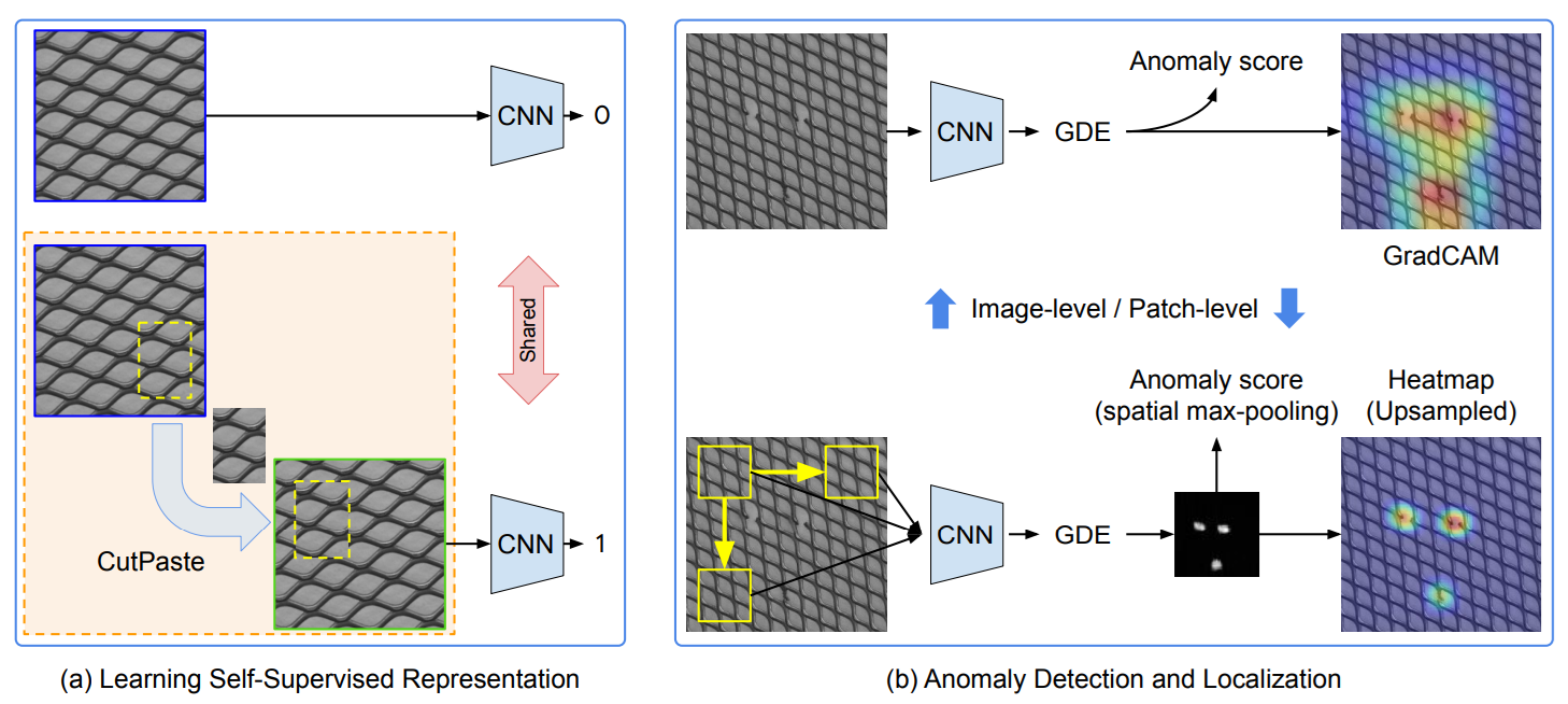
Self-supervised methods do not require manual defect labels. Instead, they create their own learning signal from normal or unlabeled images using tasks such as masking, reconstruction, contrastive learning, or synthetic anomaly generation. This helps the model learn strong representations of normal visual patterns, which can later be used to detect unusual regions during inference.

These methods are useful when abnormal samples are rare but normal images are easy to collect. Rather than learning specific defect categories, the model learns the structure of normal data so that deviations stand out as anomalies. Common examples include PatchSVDD, CutPaste and masking-based methods.

5. Unsupervised

In unsupervised VAD, the model is usually trained with only normal samples and then flags deviations at test time. This is the standard setting when abnormal data is rare, expensive, or unknown. The model does not learn defect classes, it learns normality. A recent unsupervised example is MambaAD, which learns normal visual patterns from anomaly-free images and then detects regions that deviate from that learned normality. It uses state-space modeling to capture both local details and long-range relationships in the image.

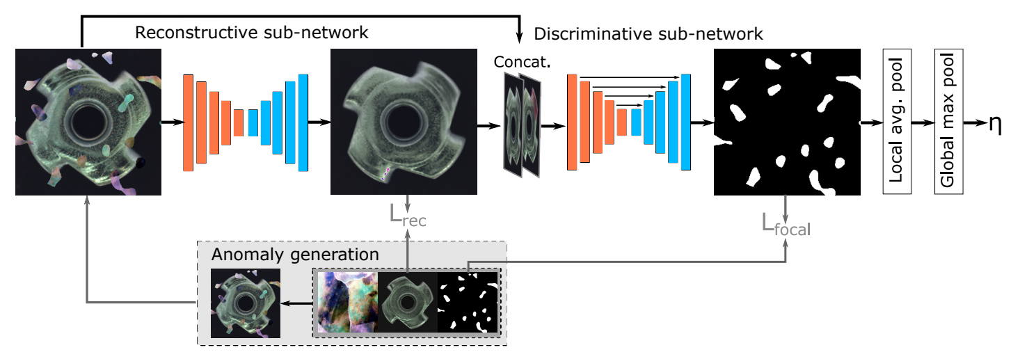
6. Reconstruction-Based Methods

Reconstruction-based methods train a model to reconstruct normal images and then use reconstruction error as the anomaly signal. The basic idea is simple, if the model has only learned normal appearance, it should reconstruct normal samples well and reconstruct abnormal regions poorly. These methods are intuitive and are still widely used for industrial surface inspection. A strong example is DRAEM, which combines reconstruction with discriminative learning so it can localize anomalies directly instead of relying only on raw reconstruction error.

7. Memory-Bank and Nearest-Neighbor Methods

Memory-bank methods store representative normal patch features and compare each test patch against that stored memory. If a patch is far from all remembered normal patches, it gets a high anomaly score. These methods are especially strong for local defects such as scratches, dents, or small texture breaks. The best-known example is PatchCore, which uses pretrained patch features, a coreset-subsampled memory bank, and nearest-neighbor search to generate both image-level anomaly scores and pixel-level heatmaps.

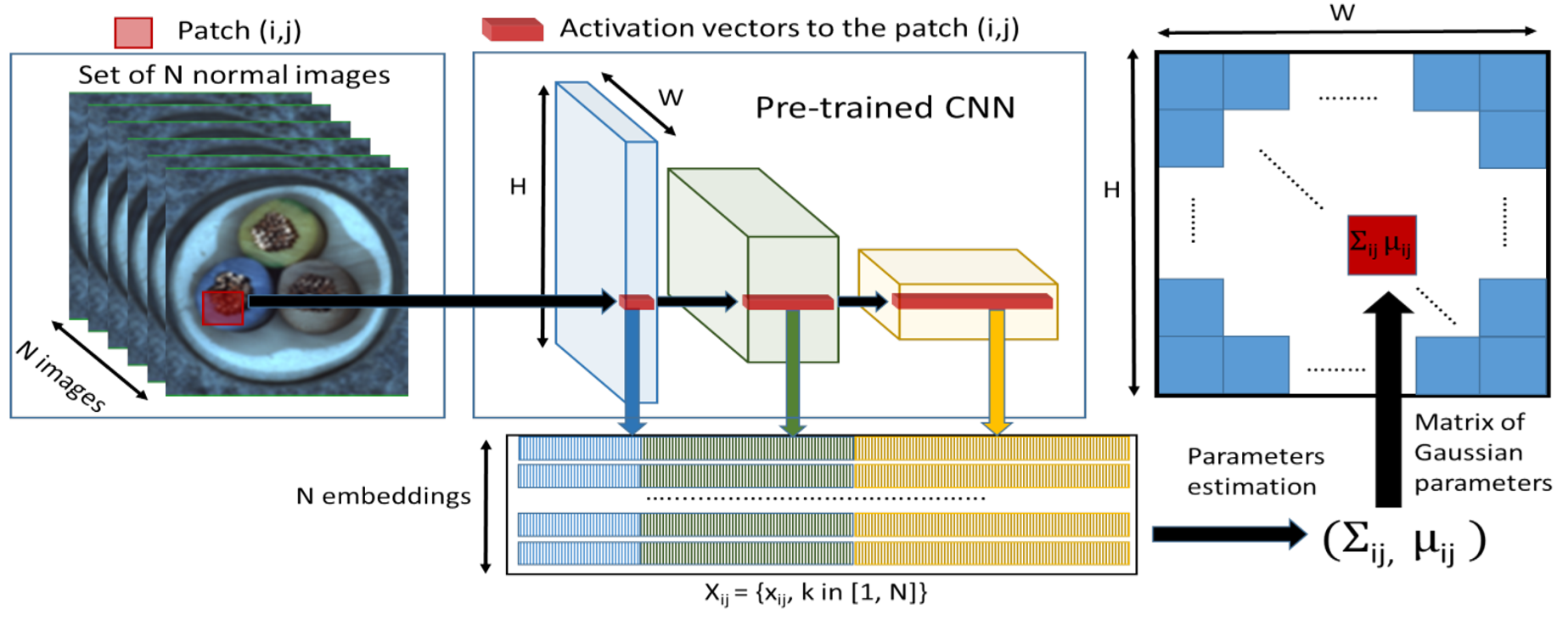
8. Distribution Modeling Methods

Distribution-modeling methods learn the statistical distribution of normal features instead of storing all of them explicitly. During inference, the model measures how strongly a test patch deviates from that learned distribution. This is useful when you want a more compact representation of normality than a full memory bank. An example of this type is PaDiM, which models patch embeddings with multivariate Gaussian distributions and uses the Mahalanobis distance for anomaly scoring and localization.

9. Knowledge Distillation Methods

Knowledge-distillation methods use a teacher-student architecture. A teacher network produces normal feature representations, and a student network is trained to imitate them on anomaly-free images. At test time, anomalies are detected where the student fails to match the teacher. This family is attractive because it can be both accurate and fast. A strong example is EfficientAD, which combines a lightweight student-teacher design with an auxiliary autoencoder branch and achieves very low-latency anomaly detection.

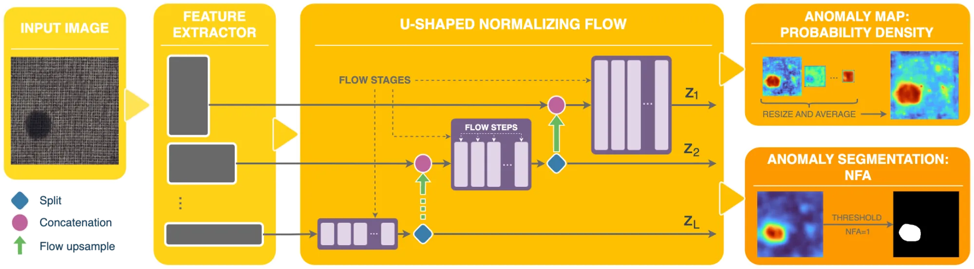
10. Flow-Based and Density-Estimation Methods

Flow-based methods explicitly model the probability distribution of normal features. If a test sample has low likelihood under that distribution, it is flagged as anomalous. These methods are a cleaner probabilistic version of the “how normal is this feature?” idea. A well-known example is FastFlow, which uses 2D normalizing flows on deep features and supports both anomaly detection and localization with strong efficiency.

11. Few-Shot Anomaly Detection

Few-shot anomaly detection works when only a small number of normal reference images are available for a target product or category. Instead of learning from a large training set, the model uses these few examples to build a baseline of normal appearance and then checks whether a new image deviates from that baseline.

This setting is useful when a new product line has very limited data, but inspection still needs to start quickly. An example of few-shot are UniVAD, DictAS and recent one SubspaceAD. It is a training-free few-shot visual anomaly detection method that uses only a few normal reference images at test time and combines component clustering, patch matching, and graph-based component modeling to detect industrial, logical, and medical anomalies.

12. Zero-Shot Anomaly Detection

Zero-shot anomaly detection aims to detect anomalies in new categories without using reference normal samples from that target category. Because no category-specific training data is available, these methods rely on external knowledge, most commonly pretrained multimodal vision-language models such as CLIP. Good examples of zero-shot anomaly detection are AnomalyCLIP, CLIP-AD, AnoCLIP, WinCLIP.

WinCLIP uses pretrained CLIP and compares image content against normal and abnormal text prompts to produce anomaly scores. Instead of using only one global image embedding, it extracts and aggregates image-level, window-level, and patch-level features, which helps it both classify whether an image is anomalous and localize where the anomaly is.

13. VLM-Based and Foundation-Model Methods

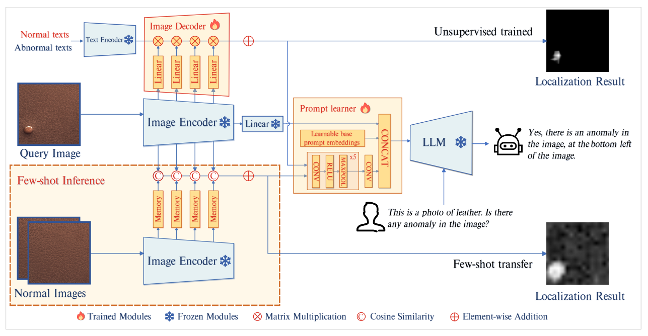
Recent methods use vision-language models and foundation models to detect anomalies with broader semantic understanding. These methods are especially useful when the anomaly is not just a small surface defect, but also a logical, relational, or scene-level problem. A good example is AnomalyGPT, which uses a large vision-language model to detect anomalies, localize them, and answer questions about what is wrong in the image.

Building an Anomaly Detection Pipeline with Roboflow Workflows

Roboflow provides two main ways to build anomaly detection applications:

• Path A - Supervised detection/segmentation: Train and deploy models like RF-DETR for known defects. This path uses Roboflow Train and Roboflow Inference for deployment.
• Path B - Unsupervised/statistical detection: Use Roboflow Workflows with embedding blocks and the Identify Outliers block to detect unknown outliers.

Path A. Supervised PCB Defect Detection

Use this strategy when the defect types are already known and can be labeled in training images. In industrial inspection, these defects can be treated as visual anomalies because they are visible deviations from the normal appearance of a product, such as scratches, cracks, missing parts, or soldering errors. However, this path is not true open-ended visual anomaly detection in the strict sense. It is actually supervised defect detection, because the model is trained to recognize specific known defect categories rather than learning normality and discovering unknown anomalies on its own.

This means the model answers a narrower question: “Does this image contain one of the known defect types I was trained to detect?” That is why this approach works best when the failure modes are already understood and stable in production. For example, in PCB defect detection for defects such as missing components, soldering defects, burn marks, or broken traces can be labeled and used to train a supervised model that directly detects and localizes them. In this example we will build the PCB defect detection model to identify "known" PCB anomalies such as "mouse bite", "missing hole", and "open circuit" Follow the steps below to build such system.

Step 1. Collect and Upload PCB Images

Collect images of PCBs that include both normal boards and boards with known defects. Upload them to a Roboflow project. For PCB inspection, Object Detection is a good choice when you want the model to locate defect regions with bounding boxes. If you need very precise defect boundaries, such as irregular scratches or burn marks, you can use Instance Segmentation instead.

Step 2. Annotate the Defects

Open the images in Roboflow Annotate and label the defect regions. For each defective PCB image, draw annotations around the defect class you want the model to learn. If the defects are very small or thin, such as fine cracks, missing solder, or tiny damaged regions, tools like SAM 3 can help speed up annotation by generating more accurate masks or region suggestions.

Step 3. Prepare the Dataset

Create a dataset version and apply preprocessing or augmentation as needed. For PCB inspection, this often includes resizing, orientation consistency, and sometimes tiling when defects are very small compared to the full image. Tiling helps the model see fine defect details at a larger relative scale during training.

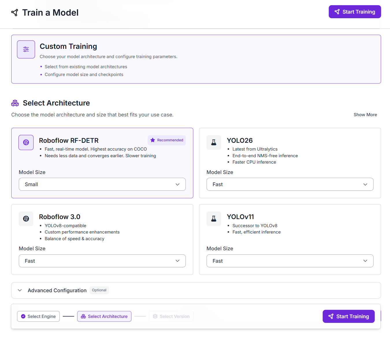
Step 4. Train the Detection Model

Train a supervised anomaly detection model on your labeled PCB defect dataset. Select RF-DETR as architecture. Once training is complete, Roboflow gives you a hosted model version that can be used inside Workflows. In your current workflow, the trained Object Detection Model block is connected directly after the image input and returns the PCB defect predictions for each frame.

Step 5. Build the Workflow

This workflow is designed to improve PCB defect inspection by combining tile-based detection with two visual outputs. The input image is first split into smaller overlapping slices so tiny PCB defects become larger relative to each tile. The sliced images are then passed through the trained detection model, and the workflow produces two outputs: one image showing detected defect boxes and confidence score, and another image showing a heatmap overlay of where detections are concentrated.

This makes the workflow useful both for direct defect inspection and for quickly understanding the spatial pattern of detections across the PCB. The Image Slicer block uses the SAHI approach to split large images into overlapping tiles so small objects are easier to detect, and the Heatmap Visualization block draws a semi-transparent blurred heat overlay based on detection positions.The blocks are arranged as follows:

• Inputs: The workflow receives one input image, named image. This is the camera frame that will be inspected.
• Image Slicer: Before detection, the input image is divided into overlapping tiles. This helps when defects are very small compared to the full PCB image, because each defect occupies more pixels inside a slice than it would in the original full frame. The Image Slicer block is specifically intended for this kind of small-object detection workflow.
• Object Detection Model: The input image is passed into your trained PCB defect decetion model. This block performs the defect detection and returns the predicted defect bounding boxes, classes, and confidence scores.
• Bounding Box Visualization: The model predictions are drawn on the image as bounding boxes so that the detected PCB defects can be seen visually.
• Label Visualization: This block adds class names and confidence labels on top of the bounding box output, creating the final annotated image.
• Heatmap Visualization: In parallel with the box-and-label path, the model predictions are also sent to the Heatmap Visualization block. This block accumulates heat based on the positions of detections and renders a semi-transparent blurred overlay on the image. In our workflow, this gives a second visual output that highlights where defect detections are concentrated on the PCB.
• Outputs: our workflow returns:
• detection_visualization from label_visualization.image — the annotated PCB image with bounding boxes and confidence label.
• heatmap_visualization from heatmap_visualization.image — the PCB image with a heatmap overlay showing defect concentration

This setup is useful because it gives two complementary views of the same inspection result. The detection visualization is helpful for checking individual predicted defects, while the heatmap visualization helps you quickly see where detections are clustering on the board.

Step 6. Deploy Locally with Roboflow Inference

You are deploying the workflow through a local Inference server running at:

http://localhost:9001

Your Python code connects to that local server, opens a webcam stream, sends frames into the workflow, receives the annotated frames back, and also prints the raw prediction data for each frame. Here's the deployment code:

import base64
import cv2
import numpy as np
import supervision as sv
from inference_sdk import InferenceHTTPClient


def decode_workflow_image(image_data):
    
    if image_data is None:
        return None

    if isinstance(image_data, dict):
        for key in ["value", "image", "base64"]:
            if key in image_data:
                image_data = image_data[key]
                break

    if not isinstance(image_data, str):
        return None

    if image_data.startswith("data:image"):
        image_data = image_data.split(",", 1)[1]

    image_bytes = base64.b64decode(image_data)
    image_np = np.frombuffer(image_bytes, dtype=np.uint8)
    image_bgr = cv2.imdecode(image_np, cv2.IMREAD_COLOR)

    if image_bgr is None:
        return None

    image_rgb = cv2.cvtColor(image_bgr, cv2.COLOR_BGR2RGB)
    return image_rgb

client = InferenceHTTPClient(
    api_url="http://localhost:9001",
    api_key="ROBOFLOW_API_KEY"
)

result = client.run_workflow(
    workspace_name="tim-4ijf0",
    workflow_id="pcb-defect-anomaly",
    images={
        "image": "l_light_11_missing_hole_05_2_600.jpg"
    },
    use_cache=True
)

print("Raw result:")
print(result)


if isinstance(result, list) and len(result) > 0:
    output = result[0]
else:
    output = result

detection_img = decode_workflow_image(output.get("detection_visualization"))
heatmap_img = decode_workflow_image(output.get("heatmap_visualization"))

print("\nPredictions:")
print(output.get("predictions"))


images = []
titles = []

if detection_img is not None:
    images.append(detection_img)
    titles.append("Detection Visualization")

if heatmap_img is not None:
    images.append(heatmap_img)
    titles.append("Heatmap Visualization")

if len(images) == 0:
    print("No images returned from workflow outputs.")
else:
    sv.plot_images_grid(
        images=images,
        grid_size=(1, len(images)),
        titles=titles,
        size=(16, 8)
    )

When you run the workflow, you will see two output images as follows.

Path B. Unsupervised / Statistical Detection

This workflow uses an embedding model to convert each image into a feature vector and then applies the Identify Outliers block to detect unusual frames statistically. It is useful when you mostly have normal samples and want to detect unknown scene changes, novelty, or unexpected visual outliers without defining defect classes in advance. However, because it works at the frame level, it is weaker for tiny local defects and does not provide pixel-level anomaly heatmaps.

Step 1. Create a Workflow

Open the Roboflow Workflow editor and create a new workflow by choosing "Build my own" option.

Step 2. Add the Embedding Block

Add a CLIP Embedding Model block (or Perception Encoder block). Wire the image input to it. This block converts each image into a numeric vector that captures the semantic content of the frame.

Step 3. Add the Identify Outliers Block

Connect the embedding output to the Identify Outliers block. Configure these parameters.

• warmup. Set to 20-50. The system collects this many embeddings before it starts flagging outliers. During warmup it is purely learning what normal looks like.
• threshold_percentile. Set to 0.05 for sensitive detection or 0.01 for strict detection. If an embedding falls below this percentile or above (1 minus this percentile), it is flagged as an outlier.
• window_size. Default is 32. Higher values make the baseline more stable but slower to adapt.

Step 4. Add a Text Display Block

After the Identify Outliers block, add a Text Display block . This block takes the original input image and overlays the outlier results as text on top of the frame. This block renders text on an image and supports dynamic parameter interpolation, styling, and positioning. This block requires two fields to be set for rendering the text. The Text field, you write the message that should appear on the image. In this workflow, the text is set as:

warming_up: {{ $parameters.warming_up }} | is_outlier: {{ $parameters.is_outlier }} | percentile: {{ $parameters.outlier_score }}

This means the block will display the live anomaly status directly on the frame. The Text Parameters field is used to map those placeholder names to actual outputs from the Identify Outliers block. In your workflow:

• warming_up is linked to steps.identify_outliers.warming_up
• is_outlier is linked to steps.identify_outliers.is_outlier
• outlier_score is linked to steps.identify_outliers.percentile

So, the Text field defines what should be shown, and the Text Parameters field tells the block where each value should come from. This allows the displayed text to update automatically for every frame.

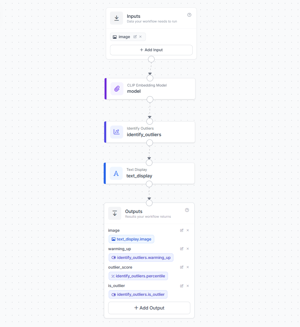
Step 5. Add Outputs

Expose the final workflow outputs so both the image and anomaly status can be returned. Your workflow should return:

• image from the Text Display block - this is the final annotated frame with the anomaly status written on top
• warming_up from the Identify Outliers block - indicates whether the system is still learning the normal baseline
• outlier_score from the Identify Outliers block using the percentile output - shows how unusual the current frame is relative to the learned baseline
• is_outlier from the Identify Outliers block - indicates whether the current frame has been flagged as an anomaly

This makes the workflow useful for both visual monitoring and structured programmatic output. The image output can be shown in a live stream, while the numeric and boolean outputs can be used for logging, alerts, or downstream automation.

Step 6. Deploy and Run

Deploy using following code on you NVIDIA device.

import cv2
from inference_sdk import InferenceHTTPClient
from inference_sdk.webrtc import WebcamSource, StreamConfig, VideoMetadata

# Initialize client
client = InferenceHTTPClient.init(
    api_url="http://localhost:9001",
    api_key="ROBOFLOW_API_KEY"
)

# Configure video source (webcam)
source = WebcamSource(resolution=(1280, 720))

# Configure streaming options
config = StreamConfig(
    stream_output=["image"],
    data_output=["outlier_score", "is_outlier", "warming_up"],
    processing_timeout=3600,
    requested_plan="webrtc-gpu-medium",
    requested_region="us"
)

# Create streaming session
session = client.webrtc.stream(
    source=source,
    workflow="anomaly-detector",
    workspace="tim-4ijf0",
    image_input="image",
    config=config
)

# Handle incoming video frames
@session.on_frame
def show_frame(frame, metadata):
    cv2.imshow("Workflow Output", frame)
    if cv2.waitKey(1) & 0xFF == ord("q"):
        session.close()

# Handle prediction data via datachannel
@session.on_data()
def on_data(data: dict, metadata: VideoMetadata):
    score = data.get("outlier_score")
    is_outlier = data.get("is_outlier")
    warming_up = data.get("warming_up")

    if score is not None:
        print(f"Frame {metadata.frame_id}: "
              f"Percentile={score} | "
              f"Outlier={is_outlier} | "
              f"WarmingUp={warming_up}")

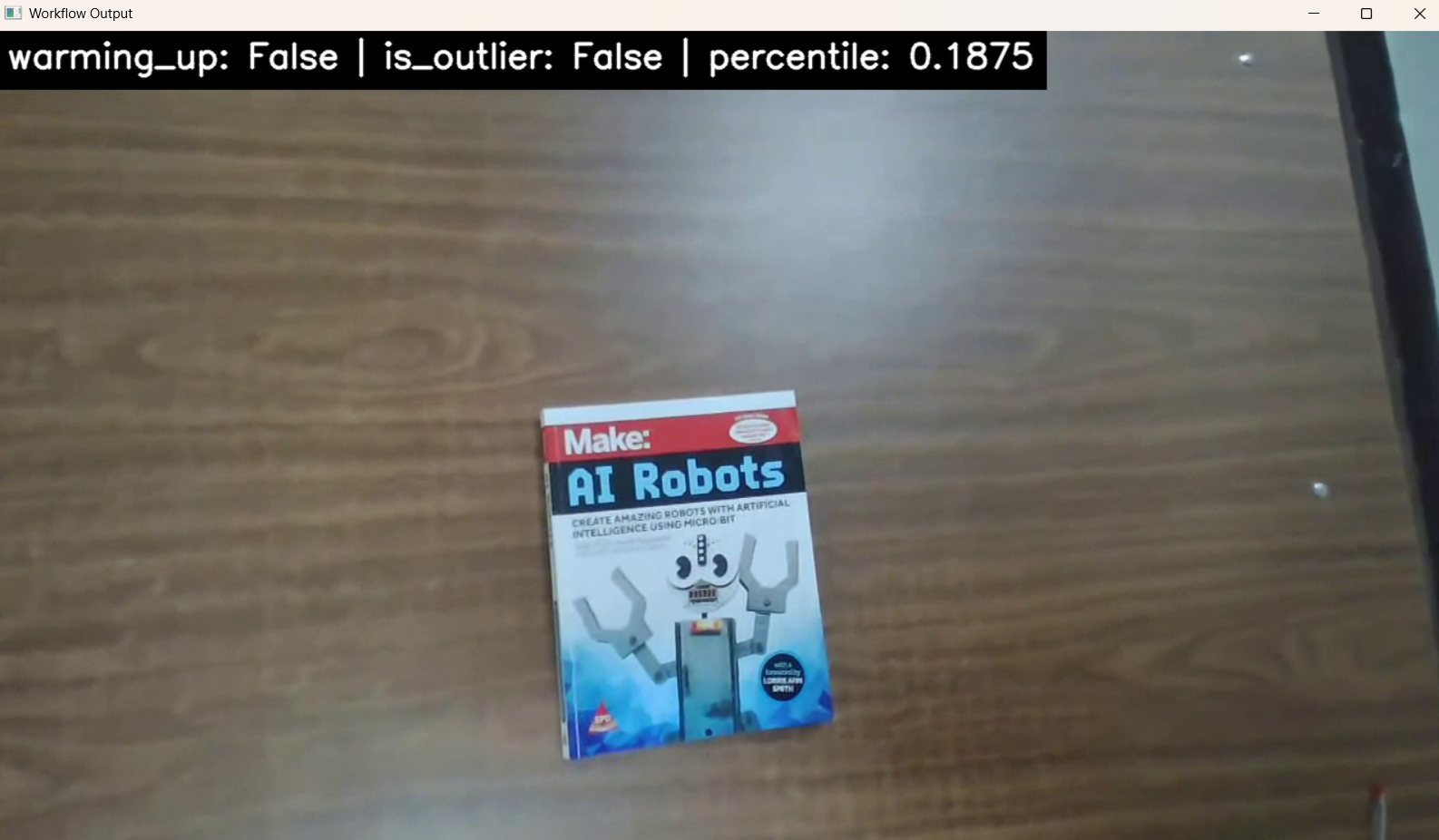
# Run the session (blocks until closed)
session.run()

When you run the workflow, you will see output similar to following.

Real-Time Deployment on NVIDIA Jetson

Roboflow supports self-hosted deployment through Roboflow Inference, its open-source edge inference server. Jetson devices with NVIDIA JetPack are supported with hardware-accelerated Docker images. A simple start path.

pip install inference-cli
inference server start

Anomaly Detection Conclusion

Anomaly detection helps a vision system notice when something looks unusual compared to normal examples. In real applications, that unusual thing could be a damaged part, a missing component, a foreign object, or any unexpected change in the image. The best method depends on the type of problem, the data you have, and how clearly you can define normal.

A good anomaly detection system starts with a good definition of normal. If the training images do not represent normal conditions well, the system may produce weak or unreliable results. Once that baseline is clear, you can build and test your first anomaly detection workflow in Roboflow on images, video, or a live camera feed.

Cite this Post

Use the following entry to cite this post in your research:

Timothy M. (Mar 12, 2026). Visual Anomaly Detection. Roboflow Blog: https://blog.roboflow.com/visual-anomaly-detection/