
A convolutional neural network (CNN) is a deep learning architecture that applies learned filters across an image to extract spatial features, then passes the results through pooling, activation, and fully connected layers to produce a classification or detection output. This explainer covers how convolution differs from standard matrix multiplication, what each layer type contributes (pooling, batch normalization, dropout, classification), and how landmark architectures like LeNet and AlexNet established CNNs as the foundation of modern computer vision.
The use of multiple hidden layers in machine learning (referred to as “deep learning”) has surpassed the performance of traditional techniques to solve various problems, particularly in the field of pattern recognition and object detection. One of the most popular architectures used in deep learning is the Convolutional Neural Network (CNN), commonly used for classification tasks.
CNNs have played a crucial role in the field of computer vision, which aims to teach machines to understand visual data. In 2012, a team of researchers from the University of Toronto developed an AI model called AlexNet, named after its main creator, Alex Krizhevsky. This model was able to achieve an unprecedented 85% accuracy in image recognition, far surpassing the 74% accuracy of the runner-up in the ImageNet computer vision contest.
The success of AlexNet was largely due to the use of CNNs, a type of neural network that mimics the way human vision works. Over the years, CNNs have become an essential component of many computer vision applications, and are now a common topic in online computer vision courses. Therefore, understanding the workings of CNNs and the CNN algorithm in deep learning is important for anyone interested in this field.
In this post, we are going to discuss:
- What convolutional neural networks are
- How convolutional neural networks work
- Common convolutional neural network architectures
Let's get started!
What is a Convolutional Neural Network?
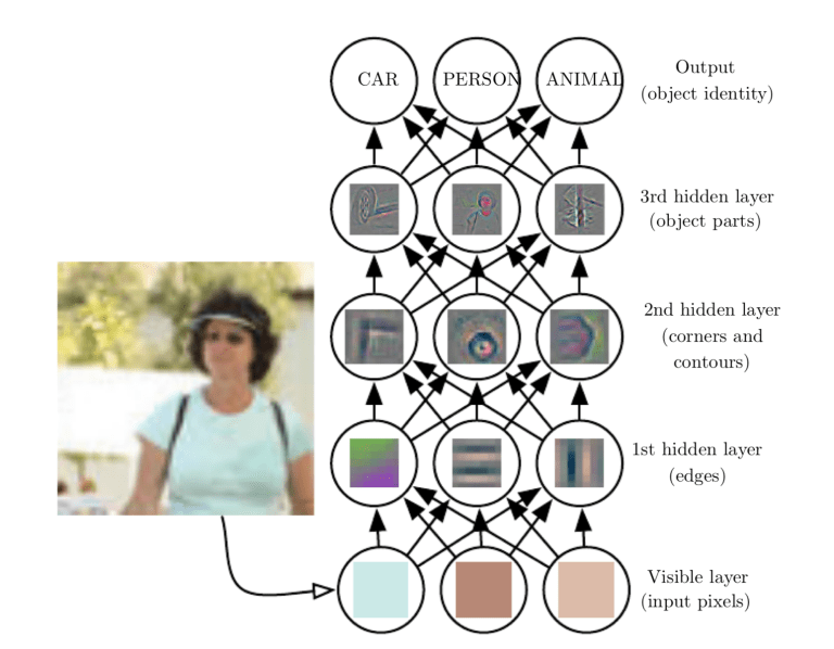
A Convolutional Neural Network (CNN) is a deep learning architecture that takes an image, applies convolutions and pooling, then goes through a fully-connected layer and activation function to return an output. This output commonly contains a classification for the contents of an image or information about the position of different objects in an image.
Unlike traditional neural networks, which primarily rely on matrix multiplications, CNNs utilize a technique called convolution. Mathematically, convolution is an operation that combines two functions to create a third function that represents how one function modifies the shape of the other. Further processing stages occur, including pooling and passing through fully-connected layers and an activation function to return a prediction. Below, you can see a typical architecture of a CNN.
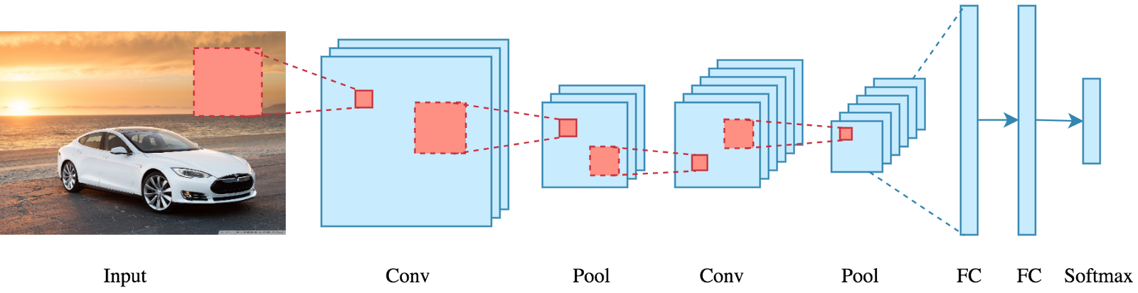
The convolutional layers within a CNN, through the process of convolution, effectively scan the image and extract key features such as edges, textures, and shapes. These features are then passed through multiple layers and processed using techniques such as pooling and activation functions, leading to a compact, yet informative, representation of the original image. This compact representation is then used as input for the fully connected layers of the network, which make the final predictions.
While understanding the mathematical details behind convolution can be helpful, it is not essential to grasp the overall concept of a CNN.
At a high level, a CNN is designed to take in an image and convert it into a representation that a neural network can understand, while still preserving important features that will enable accurate predictions.
CNNs vs. Feed-Forward Neural Nets
To properly understand CNNs in context, it is important to consider their antecedent: feed-forward neural networks.
A feedforward neural network is a type of neural network that processes data in a single pass, with the input being passed through multiple layers before reaching the output. When it comes to image processing, feedforward networks have a major limitation: the risk of overfitting.
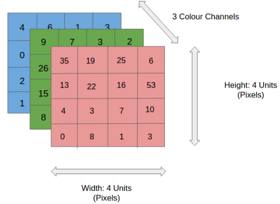
An image can be represented as a matrix of numbers with a shape of (rows * columns * number of channels). A typical real-world image would be at least 200 * 200 * 3 pixels in size. One approach to feeding an image into a feedforward neural network would be to flatten the image into a 1D matrix. However, this would require a large number of neurons and a corresponding number of weights at the first hidden layer. This leads to a large number of parameters, which can increase the risk of overfitting.
In contrast, convolutional neural networks approach image processing in a different way. Rather than flattening the image and processing it in one pass, CNNs process small patches of an image at a time and move across the entire image. This allows the network to learn essential features of the image, while using fewer neurons and fewer parameters. This approach makes CNNs more efficient and less prone to overfitting than feedforward neural networks.
How Do Convolutional Neural Networks Work?
Before diving into the inner workings of convolutional neural networks, it is important to understand the basics of images and how they are represented.
An image can be represented as a matrix of pixel values, with each pixel having a specific color value. RGB images, which are the most commonly used type of images, have three planes representing the Red, Green, and Blue color channels. Grayscale images, on the other hand, have only one plane. This plane represents the intensity of the pixel.
The number of pixels in an image determines its resolution, with a higher resolution image having more pixels and thus more detailed information.
Now we have discussed the background we need to dive into how CNNs work. Let’s walk through an example using grayscale images since their structure is not as complex as RGB images.
What is a Convolution?
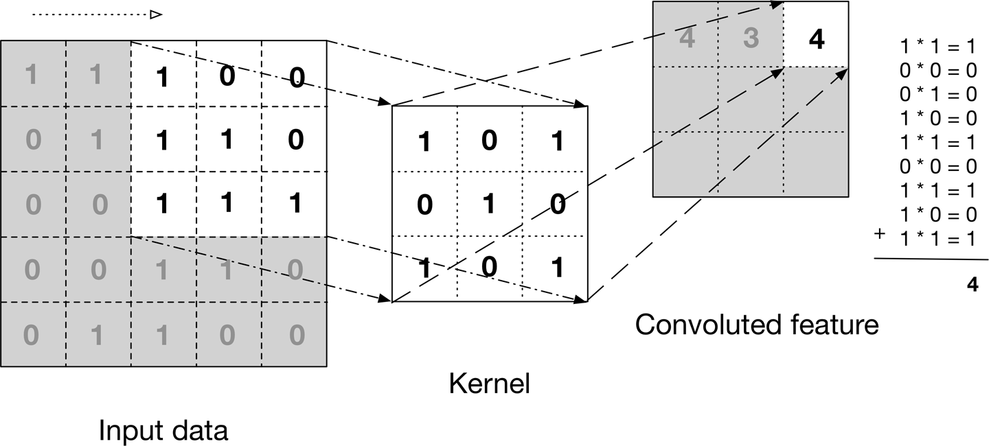
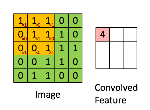
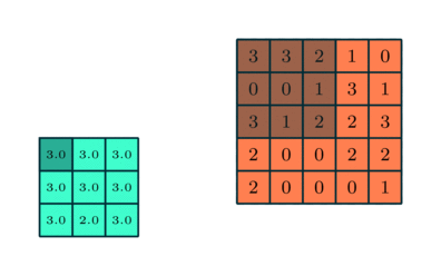
A convolution is a process in which a small matrix, known as a filter or kernel, is applied to an input image in order to extract important features. The filter is moved across the image, with the values at each position being multiplied by the corresponding values in the image and the results being summed together.
This process results in a “convolved feature”, which is then passed on to the next layer for further processing. Here is an animation of the process being applied to a 5x5 grid of pixel data:
Convolutional neural networks are composed of a series of interconnected layers of artificial “neurons”. These artificial neurons are mathematical functions that take in multiple inputs, weigh them, and return an activation value.
The first layer of the ConvNet is responsible for identifying basic features such as edges, corners, and other simple shapes. As the image is passed through successive layers, the network is able to detect more complex features, such as objects and faces, by building upon the information gathered from previous layers. As the image is processed deeper into the network, it can identify even more complex features such as objects, faces, etc.
The final convolution layer of a convolutional neural network generates an “activation map”. In classification tasks, for example, a classification layer uses this map to determine the likelihood that the input image belongs to a specific "class".
This likelihood is represented as a set of confidence scores, with values ranging from 0 to 1. For example, if the ConvNet is designed to recognize cats, dogs, and horses, the output of the final layer will be the probabilities that the input image contains one of those animals. The higher the value, the more likely it is that the image contains the corresponding class.
CNNs in Object Detection
CNNs can be used for object detection, a task that involves locating and identifying objects in an image or video. The output of a CNN in this case would be a set of bounding boxes around the objects in the image, along with class labels and confidence scores indicating what each object is and how certain the network is of its predictions.
There are different approaches to using CNNs for object detection, but a common one is to use a two-stage framework, such as the popular R-CNN (Regions with Convolutional Neural Networks) family of models. In the first stage, the network is used to propose candidate object regions in the image, called "region proposals".
These region proposals are then processed by a second stage, where a fully connected network is used to classify the objects in the regions and refine the bounding boxes. More recent approaches, such as YOLO (You Only Look Once) and RetinaNet, use a single-stage approach, where the network predicts the bounding boxes, class labels, and confidence scores directly from the input image in a single pass. These models tend to be faster than the two-stage approaches, but often have slightly lower accuracy.
Regardless of the specific architecture, the main idea behind using CNNs for object detection is to leverage the convolutional layers to extract rich, discriminative features from the image, and then use these features to make predictions about the objects in the image.
Layers in Convolutional Neural Networks
In this section, we will provide a comprehensive overview of the layers that are commonly utilized in building convolutional neural network architectures. We will examine the various types of layers that make up CNNs: the pooling layer, activation layer, batch normalization layer, dropout layer and classification layer. Let’s begin!
Pooling Layer
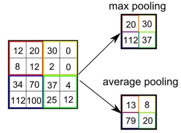
The Pooling layer, similar to the Convolutional Layer discussed earlier, reduces the spatial size of the convolved features within a convolutional neural network.
This reduction in spatial size is achieved by down-sampling the convolved features. This serves the dual purpose of both decreasing the computational power required to process the data and also increasing the level of abstraction in the features.
There are two common types of pooling techniques used in CNNs: average pooling and max pooling.
Max pooling reduces the spatial size of the convolved features by down-sampling. It works by selecting the maximum value of a pixel from a portion of the image covered by the kernel.
This technique not only reduces the computational power required to process the data but also serves as a noise suppressant, discarding noisy activations and performing de-noising along with dimensionality reduction.
On the other hand, average pooling returns the average of all the values from the portion of the image covered by the kernel. While it also serves the purpose of dimensionality reduction, it lacks the noise suppression capabilities of max pooling.
As a result, max pooling is generally considered to be more effective and robust in practice, providing better performance than average pooling. The choice between these two techniques largely depends on the specific requirements of the task and the noise level in the dataset.
Activation Function Layer
The activation function layer helps the network learn non-linear relationships between the input and output. It is responsible for introducing non-linearity into the network and allowing it to model complex patterns and relationships in the data.
The activation function is typically applied to the output of each neuron in the network. It takes in the weighted sum of the inputs and produces an output that is then passed on to the next layer.
The most commonly used activation functions in CNNs are:
- Rectified linear unit (ReLU)
- Sigmoid
- Hyperbolic tangent (tanh)
ReLU is a popular choice in CNNs because it is computationally efficient and tends to produce sparse representations of the input data. It returns the input if it is positive, and returns 0 if it is negative. Sigmoid and tanh are other nonlinear functions but are not as commonly used as ReLU in CNNs because they can produce gradients close to 0 when the input is large. The activation function layer can be thought of as the "brain" of the CNN, where the input is transformed into a meaningful representation of the data. It is a fundamental component.
To learn more about activation functions, check out our comprehensive guide to activation functions.
Batch Normalization Layer
The Batch Normalization (BN) layer is commonly used in convolutional neural networks to normalize the input of each neuron to have zero mean and unit variance. This helps to stabilize the learning process and prevent the problem of internal covariate shift, which occurs when the distribution of the inputs to a layer changes during the training process.
BN normalizes the output of each neuron using the mean and standard deviation of the batch of input data and is usually applied after the convolutional and fully connected players.
The Batch Normalization layer has several positive effects on CNNs:
- BN can accelerate the training process by reducing the internal covariate shift and allowing for higher learning rates.
- BN helps to regularize the model, making it less prone to overfitting.
- BN has been shown to improve the generalization performance of CNNs, allowing them to achieve better performance on unseen data.
- BN helps to reduce the number of hyperparameters that need to be tuned, such as the learning rate. This will result into a simplification of the training process and an improvement on generalization.
- BN allows a model to be less sensitive to the initial values of the weights.
In summary, Batch Normalization is a powerful technique that is widely used in CNNs to stabilize the learning process and improve the performance of the model. It normalizes the inputs to each neuron, reducing the internal covariate shift and regularizing the model, which leads to better generalization performance.
Dropout Layer
The dropout layer uses a regularization technique to prevent overfitting. It works by randomly setting a proportion of input units to zero during each training iteration, effectively "dropping out" those units and preventing them from contributing to the forward pass.
This process forces the network to learn multiple independent representations of the input, making it more robust to changes in the input data and reducing the chances of overfitting. Dropout is typically applied to the fully connected layers of a CNN, but can be applied to any layer.
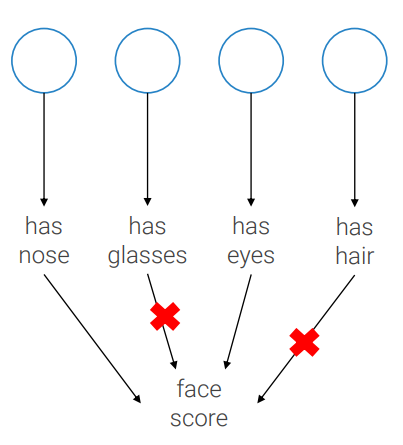
The idea of dropout was inspired by Hinton and his bank:
“I went to my bank. The tellers kept changing and I asked one of them why. He said he didn’t know but they got moved around a lot. I figured it must be because it would require cooperation between employees to successfully defraud the bank. This made me realize that randomly removing a different subset of neurons on each example would prevent conspiracies and thus reduce overfitting.”
Say we want to detect a face. In general, the faces do not always have all the face attributes like nose, eyes, eyes, etc.. In general, something could be missing. So for example I would like to train my network also for faces with an occluded eye. So it is a good idea to not have all the features that co-adapt but randomly learn a subset of these features to be able to generalize better on unseen data, so to force my face detector to work also when only some of the attributes are present.
Classification Layer
The classification layer is the final layer in a CNN. This layer produces the output class scores for an input image. There are two main types of classification layers used in CNNs: fully connected layers and global average pooling layers.
A fully connected (FC) layer is a standard neural network layer that connects all the neurons in the previous layer to all the neurons in the current layer. The output of a FC layer is computed by applying a weight matrix and a bias vector to the input, followed by an activation function. The FC layer is then connected to a softmax activation to produce the class scores.
The advantage of using fully connected layers is that they allow the network to learn complex decision boundaries between classes. On the other hand, these layers can lead to overfitting and require a large number of parameters. To counter these issues, global average pooling (GAP) has been introduced.
A global average pooling layer is a type of pooling layer that reduces the spatial dimensions of the feature maps by taking the average value of each feature map. The output of the GAP layer is a 1D vector of size equal to the number of feature maps. The GAP layer is connected to a fully connected (FC) layer with softmax activation to produce the class scores.
The advantage of using GAP layers is that they are less prone to overfitting and require fewer parameters. However, GAP layers do not allow the network to learn complex decision boundaries between classes.
In summary, fully connected layers are good for complex decision boundaries but require many parameters and can lead to overfitting. GAP layers are less prone to overfitting, but they are less able to learn complex decision boundaries.
Well-Known CNN Examples
Let's discuss some of the prevalent implementations of convolutional neural networks, with reference to both older and more modern CNNs.
LeNet
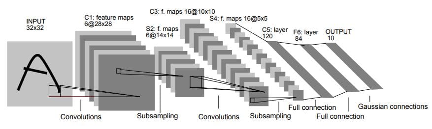
LeNet was first proposed by Yann LeCun in 1998 for handwritten digit recognition. It is considered one of the first successful CNNs and was the foundation for many subsequent CNN architectures/
The architecture of LeNet consists of several layers, including:
- Two convolutional layers, each followed by a max-pooling layer, which are used to extract features from the input image.
- Two fully connected layers, also known as dense layers, are used to classify the features.
The first convolutional layer has 6 filters of size 5x5, and the second convolutional layer has 16 filters of size 5x5. The max-pooling layer reduces the spatial dimensions of the feature maps by taking the maximum value in each window of size 2x2.
The first fully connected layer has 120 neurons and the second fully connected layer has 84 neurons. The last layer is a fully connected layer that has 10 neurons, one for each digit class.
LeNet is a relatively simple architecture but it is still used today as a starting point for many image classification tasks. However, LeNet is not as powerful as many more recent architectures.
AlexNet
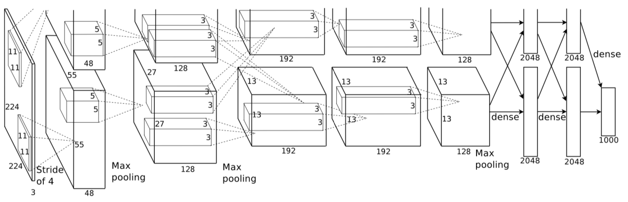
AlexNet was proposed by Alex Krizhevsky, Ilya Sutskever, and Geoffrey Hinton in 2012. It was the winning model of the ImageNet Large Scale Visual Recognition Challenge (ILSVRC) in 2012. AlexNet was the first CNN to surpass the performance of traditional, hand-designed models on this benchmark.
The architecture of AlexNet consists of several layers, including:
- Five convolutional layers, each followed by a max-pooling layer, which are used to extract features from the input image.
- Three fully connected layers, also known as dense layers, which are used to classify the features.
The first two convolutional layers have 96 filters of size 11x11, the next two convolutional layers have 256 filters of size 5x5 and the last convolutional layer has 384 filters of size 3x3. The max-pooling layer reduces the spatial dimensions of the feature maps by taking the maximum value in each window of size 2x2. The first fully connected layer has 4096 neurons, the second fully connected layer has 4096 neurons and the last layer is a fully connected layer that has 1000 neurons, one for each class of the ImageNet dataset.
AlexNet introduced several key innovations that allowed it to achieve state-of-the-art performance at the time, such as the use of the ReLU activation function, data augmentation and dropout regularization. It also had a much larger capacity than LeNet and it was able to learn more complex features from the images.
At the time, AlexNet was widely considered as a breakthrough in the field of computer vision and has inspired many of the architectures that followed.
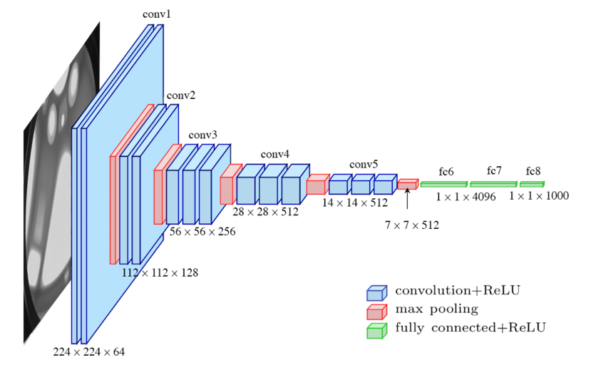
VGGNet
VGGNet is a convolutional neural network architecture developed by the Visual Geometry Group (VGG) at the University of Oxford. It was introduced in a 2014 paper by Karen Simonyan and Andrew Zisserman, and it was used to win the ILSVRC-2014 competition.
VGGNet is known for its simplicity while achieving good performance in image classification tasks. It consists of a stack of convolutional and max-pooling layers followed by fully connected layers. The key feature of VGGNet is its use of very small convolutional filters (3x3) with a very deep architecture (up to 19 layers). This architecture was later modified and used as a backbone for various computer vision tasks like object detection and image segmentation.
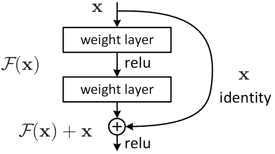
ResNet
One of the main challenges in training very deep neural networks is the problem of vanishing gradients, where the gradients (used for updating the parameters during training) become very small and training becomes slow. ResNet (Residual Neural Network), developed by Microsoft Research in 2015, addresses this problem by introducing the concept of “residual connections”.
A residual connection is a shortcut connection that bypasses one or more layers and allows the gradient to flow directly to earlier layers. This allows ResNet to train much deeper networks than previous architectures without suffering from the vanishing gradient problem.
ResNet architectures are characterized by their depth. The original ResNet had 152 layers. More recent versions, like ResNet-50, ResNet-101 and ResNet-152 have 50, 101, 152 layers respectively. ResNet has become a popular choice as a backbone for various computer vision tasks, such as object detection, semantic segmentation and image classification.
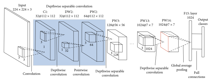
MobileNet
MobileNet, developed by Google in 2017, was specifically designed for use on mobile and embedded devices with limited computational resources. MobileNet uses depth-wise separable convolutions to reduce the number of parameters and computational cost while maintaining good accuracy.
A depth-wise separable convolution applies a single convolutional filter to each input channel (depth-wise convolution) and then applies a pointwise convolution (1x1 convolution) to combine the results. This approach reduces the number of parameters and computation required compared to standard convolutional layers.
The MobileNet architecture is designed to be lightweight and efficient, hence being well-suited for deployment on mobile and embedded devices with limited memory and processing power.
The model is available in several versions, with different levels of complexity and accuracy. MobileNet V1, V2 and V3 are the most popular versions. The most recent version, MobileNet V3, is considered to be the most efficient, with a good balance of accuracy and efficiency.
MobileNet has been used in a wide range of applications, such as object detection, semantic segmentation, and image classification, and it's been used as a backbone for many computer vision tasks, such as face recognition, object tracking and many more.
Conclusion
Convolutional Neural Networks are a type of deep learning architecture that has become widely used in computer vision tasks such as image classification, object detection, and semantic segmentation. CNNs have several advantages over traditional computer vision methods, including:
- Robustness to translation and rotation: CNNs are able to learn features that are robust to small changes in the position and orientation of the objects in the image, which makes them well-suited for tasks such as object detection and semantic segmentation.
- Handling large amounts of data: CNNs are able to learn from large amounts of data, which makes them well-suited for training on large datasets such as ImageNet.
- Transfer learning: CNNs trained on large datasets such as ImageNet can be fine-tuned on smaller datasets, which can significantly reduce the amount of data and computational resources required to train a model for a specific task.
On the other hand, CNNs also have some limits and challenges, including:
- Computational cost: CNNs require a significant amount of computational resources to train and deploy, which can be a limiting factor for deployment on mobile and embedded devices.
- Overfitting: CNNs can be prone to overfitting when the amount of data is limited, which can lead to poor performance on unseen data.
- Explainability: CNNs are often considered to be black boxes, making it difficult to understand how they are making decisions and to identify potential errors.
Cite this Post
Use the following entry to cite this post in your research:
Petru P.. (Feb 10, 2023). What is a Convolutional Neural Network?. Roboflow Blog: https://blog.roboflow.com/what-is-a-convolutional-neural-network/