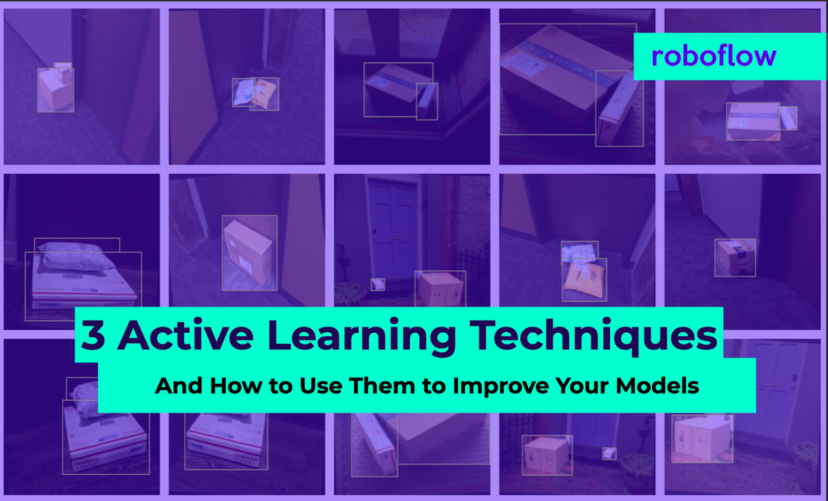
Machine learning algorithms are exceptionally data-hungry, requiring thousands – if not millions – of examples to make informed decisions. Providing high quality training data for our algorithms to learn is an expensive task. Active learning is one strategy that optimizes the human labor required to build effective machine learning systems.
Further discussion on our YouTube (don't forget to like & subscribe!)
What is Active Learning?
Active learning is a machine learning training strategy that enables an algorithm to proactively identify subsets of training data that may most efficiently improve performance. More simply – active learning is a strategy for identifying which specific examples in our training data can best improve model performance. It's a subset human-in-the-loop machine learning strategies for improving our models by getting the most from our training data. See how you can use Roboflow Active Learning to automate this process in your vision pipeline.
An Example of Active Learning in Practice
Imagine you are building a computer vision model to identify packages left on your doorstep in order to send you a push alert that you have received mail. Packages come in a wide array of shapes, sizes, and colors. Say your training data contains 10,000 example images: 600 images of packages that are brown cardboard boxes, 300 images of flat and puffy white envelopes, and 100 images of yellow boxes.
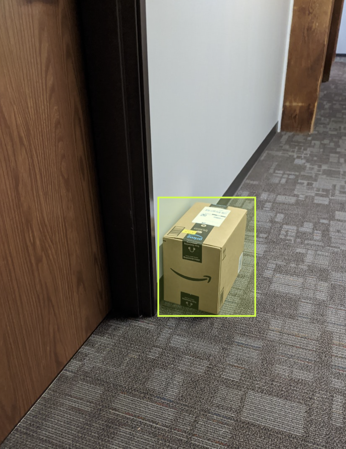
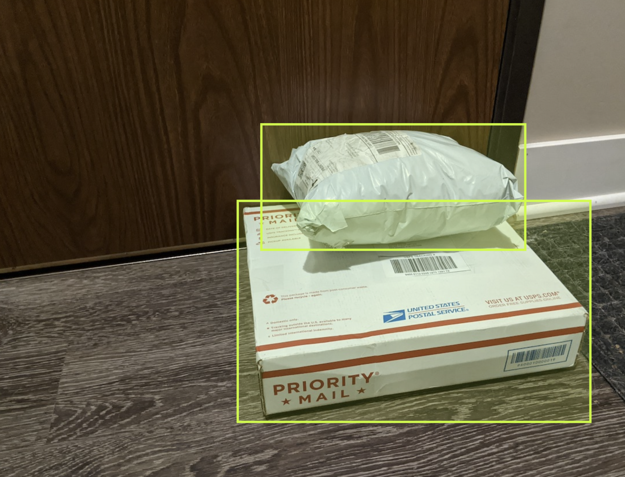
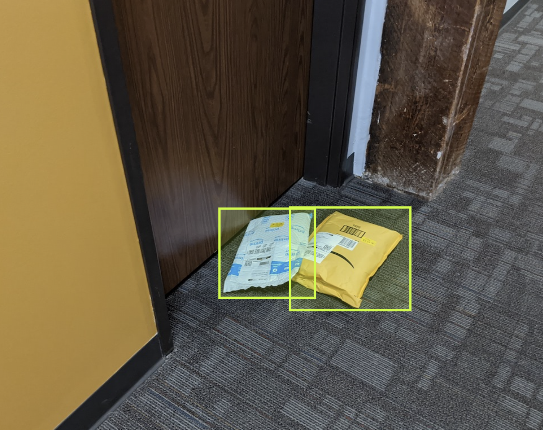
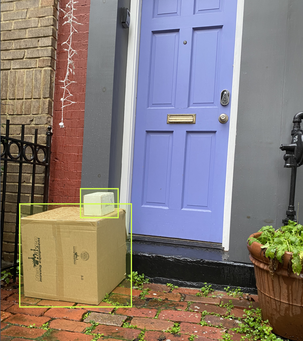
Imagine building a computer vision model to identify packages. (Source: Packages dataset.)
Moreover, each of these boxes could be left on your porch in a different spot, the weather could vary the brightness and darkness on a given day, and the boxes themselves can vary in size. An ideal dataset will have a healthy diversity of variation to capture all possible circumstances: a small yellow box on the left side of your porch during the day to a white envelope on the the right side on a cloudy day (and everything in between, in theory).
We'll say you want to develop a model quickly yet accurately, so you err on the side of labeling a 1,000 images subset of your full 10,000 images, assessing model performance, and then labeling additional data. (Did you know that you can label images in Roboflow?)
Which 1,000 images should you label first?
Intuitively, you'd opt to label some number of each of our hypothetical package classes: brown boxes, white envelopes, and yellow boxes. Because our model cannot learn what, say, a brown box is without seeing any examples of it, we need to be sure to include some number of brown boxes in our training data. Our model would go from zero percent mean average precision on the box class to some non-zero mAP on the brown box class once having examples.
The intuitive decision to ensure our first 1,000 images include examples from each class we want our model to learn is, in effect, one type of active learning. We've narrowed our training data to a set of images that will best improve model performance.
This same concept extends to other attributes of the boxes in our image dataset. What if we selected 300 brown box examples, but every brown box example was a perfect cube? What if we selected all 100 yellow box examples, but our yellow boxes were always delivered on sunny, bright days? Again, our goal should be to create a dataset that includes variation in each of our classes so our model can best learn about packages delivered of any size, in any position, and in any weather condition.
Types of Active Learning
There are multiple methods by which we could aid our model's learning from our initial training data. These methods may include generating additional examples from our training data or determining which subset of examples are most useful to our model. At our core, we're aiming to identify which samples (subset) from a full population (our training data) can best aid model performance.
Sampling which examples are most helpful to our model can follow a few strategies: pool-based sampling, stream-based selective sampling, and membership query synthesis.
All active learning techniques rely on us leveraging some number of examples with ground truth, accurate labels. That is, we inevitably need to human label a number of examples. The active learning techniques differ in how we use these known, accurate examples to identify additional unknown, useful examples from our dataset.
To evaluate these different active learning techniques, pretend we have some "active learning budget" we can spend on paying to perfectly label examples from our package dataset. Now, given all active learning techniques require we already have some number of examples with accurate labels, let's pretend we were given 1,000 perfectly labeled examples to start. We'll also pretend we have 1,000 "active learning credits" in our budget to spend on getting the perfect labels for the an additional 1,000 unlabeled package images.
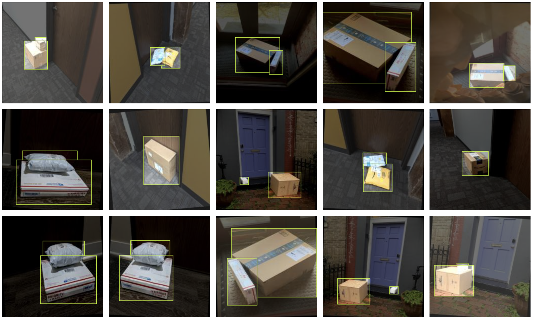
Thus, the question is: how should we spend our budget to identify the next most helpful examples to improve our model's performance.
Let's break each active learning technique down, and how they may spend our budget on our theoretical package example.
Pool-Based Sampling
Pool-based sampling is an active learning technique wherein we identify the "information usefulness" of all given examples, and then select the top N examples for training our model. Said another way, we want to identify which examples are most helpful to our model and then include the best ones.
Pool-based sampling is perhaps the most common technique in active learning, though it is fairly memory intensive.
To relate this to how we spend our "active learning cash budget," consider the following strategy. Remember, we already have an allotment of 1000 perfectly human labeled package examples. We could train a model on 800 labeled examples and validate on the remaining 200 labeled examples. With this model, we could assume that the model's lowest predicted precision examples are the ones that are going to be most helpful to improving performance. That is, the places where our model was most wrong in the validation set may be images that are most useful for future training.
So how do we spend our pretend 1,000 active learning credits with pool-based sample? We could run our model on the remaining 9,000 package images. We'll then rank our images by lowest predicted label probabilities: images where no packages were found (0 percent precision) or packages were found with low confidence (say, sub 50 percent precision). We'll spend our 1,000 active learning credits on the 1,000 lowest ranking examples to magically have perfect labels for them. (We may also want to evaluate our mAP per class to select examples weighted towards lower performing package classes.)
Voila! We've optimized our active learning budget to work on the images that will best improve our model.
Stream-Based Selective Sampling
Stream-based selective sampling is an active learning technique where, as the model is training, the active learning system determines whether to query for the perfect ground truth label or assign the model-predicted label based on some threshold. More simply, for each unlabeled example, the active learning agent says, "Do I feel confident enough to assign the model to this myself, or should I ask for the answer key for this example?"
Stream-based selective sampling can be exhaustive search – as each unlabeled example is examined one-by-one – but it can cause us to blow through our active learning budget depending on if the model queries for the true ground truth label too many times.
Let's consider what this looks like in practice for our packages dataset and 1,000 credit active learning budget. Again, remember we start with a model that we've trained on our first 1,000 perfectly labeled examples. Stream-based active learning would then go through the remaining 9,000 examples in our dataset one-by-one and, based on a confidence threshold of predicted labels, the active learning system would decide whether or not to spend one of our active learning credits for a perfectly labeled example for that given image.
But wait a minute: what if our active learner requests labels for more than 1,000 examples? This is exactly the disadvantage of stream-based selective sampling: we may go beyond our budget if our model determines that more than 1,000 examples require a true ground truth label (relative to our confidence threshold). Alternatively, if our budget is truly capped at 1,000, our stream-based sample may not make its way through the full remaining 9,000 examples – only some random first N that stayed within our budget. (This is undesired as we have not optimized the spend of our active learning budget against unlabeled examples.)
Membership Query Synthesis
Membership query synthesis is an active learning technique wherein our active learning agent is able to create its own examples based on our training examples for maximally effective learning. In a sense, the active learning agent determines it may be most useful to, say, create a subset of an image in our labeled training data, and use that newly created subset image for additional training.
Membership query synthesis can be highly effective when our starting training dataset is particularly small. However, it may not always be feasible to generate more examples. Fortunately, in computer vision, this is where data augmentation can make a huge difference.
For example, pretend our package dataset has a shortage of yellow boxes delivered on dark and cloudy days. We could use brightness augmentation to simulate images in lower light conditions. Or, alternatively, imagine many of our brown box images are always on the left side of the porch and close to our camera. We could simulate zooming out or randomly crop the image to alter perspective in our training data.
We could relate this to spending our 1,000 active learning credits by saying we spend a credit every time we generate a new image. Notably, we would need an intelligent way to determine which types of images should be generated.
This is where examining a Dataset Health Check of our data would go a long way: we may want to over index on generating yellow box images as, in our example, we only had 100 of them to start. Moreover, knowing the general position of our bounding boxes in the images would help us realize if our delivered packages skew towards one part of our porch.
Active Learning Tips
The principle question of active learning becomes: how can we identify which data points we should prioritize for (re)training? More simply put, which images will improve our model's capabilities faster.
Model failure comes in multiple forms. Let's return to the package detection model example. Perhaps our model identifies objects on our doorstep that are not packages as packages – false positive detections. Perhaps our model fails to identify that there was a package on our doorstep – false negatives. Perhaps our model identifies packages, but it is not very confident in those detections.
In general, there should always be continued monitoring (and data collection) of our production systems. Here's a few strategies we can employ to improve continuous data collection.
We've discussed active learning on Roboflow YouTube too. Subscribe: https://bit.ly/rf-yt-sub
1. Continuously Collect New Images at Random
In this example, we would sample our inference conditions on a regular interval regardless of what the model saw in those images. Pretend we have a model that is running on a video feed. With continued random dataset collection, we may grab every 1000th frame and send it back to our training dataset.
Random data collection has the advantage of helping catch false negatives, especially. Because we may not have known where the model failed, a random selection of images may include those failure cases.
On the other hand, random data collection is, well, random. It's not particularly precise, and that can result in searching a haystack of irrelevant images for our needle of insight.
2. Collect New Images Below A Given Confidence Threshold
When a model makes a prediction, it provides a confidence level for that prediction. We can set some acceptable confidence criteria for model predictions. If our model's prediction is below that threshold, it may be a good image to send back to our training dataset.
This strategy has the advantage of focusing our data collection on places that may include model failure more clearly. It's an easy, low-risk optimization for improving our data collection.
However, this strategy won't catch all false positives or any false negatives. False positives could, in theory, be so confidently false from the model that they exceed our threshold. False negatives would not have a confidence associated; there's no prediction in these cases.
3. Solicit Your Application's Users to Verify Model Predictions
Depending on the circumstances of your model, you may be able to leverage users that are interacting with the model for their confirmation or rejection of model outputs. Pretend you're building a model that helps pharmacists count pills. Those pharmacists may have oversight into the model's predictions compared to their perceived counts. The application using the vision model could include a button to say that a given count looks incorrect, and that sample could be sent back for continued training. Even better, when a user doesn't say something looks incorrect, that sample could be used for continued retraining in the form of affirmation of model performance.
The advantage to this strategy is that it includes a human-in-the-loop at the time of production usage, which significantly reduces the overhead to checking model performance.
Of course, this strategy only works if a model is interacting with end user input, which may not be the case for things like remote sensing or monitoring. In any case, systems that remove human need to review images or video commonly have a phase of blending model and human inference before going fully autonomous where this strategy can be employed.
Incorporating Active Learning into Your Applications
All of the above strategies rely on automated ways of sending images of interest back to a source dataset – which is made possible using pip install roboflow.
Roboflow also includes an Upload API wherein you can programmatically send problematic images or video frames back to your source dataset. (Note: in cases where your model is running completely offline, you can cache the images until the system may have a regular interval of external connectivity to send images.)
In addition, any model trained with Roboflow includes the model confidence per image (classification) or per bounding box (object detection). These confidences can be used for inferring which images may be good ones to use for continued model improvement.
As always, happy building!
Applying Active Learning on Your Datasets
Fortunately, many of the active learning techniques reviewed here are not mutually exclusive. For example, we can both create a "information usefulness" score of all of our images as well as generate additional images that best assist in model performance.
As is the case in most machine learning problems, having a clear understanding of your data and being able to rapidly prototype a new model based on added ground truth labels is essential.
Roboflow is purpose-built for understanding your computer vision dataset (class balance, annotation counts, bounding box positions), conducting image augmentation, rapidly training computer vision models, and evaluating mean average precision on validation vs test sets as well as by class.
Roboflow makes it easy to continue to collect images from your deployed production conditions with our Active Learning feature so you can programmatically add new examples from real inference conditions.
Cite this Post
Use the following entry to cite this post in your research:
Joseph Nelson. (Sep 1, 2024). What is Active Learning? The Ultimate Guide.. Roboflow Blog: https://blog.roboflow.com/what-is-active-learning/
