
Feature matching in computer vision refers to the process of finding corresponding keypoints between two images of the same scene or object. These keypoints are distinctive image features, such as corners, edges, blobs, or regions with significant intensity changes that can be reliably identified in different images, even if those images have undergone transformations like scaling, rotation, or changes in illumination.
The primary goal of feature matching is to identify the same physical points or objects across different images, which is fundamental for tasks like object recognition, image alignment, 3D reconstruction, and motion tracking.
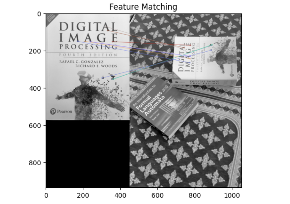
The image below shows a feature matching process, where keypoints from two images of the same book (regardless of its orientation and scale in the images) are detected and matched. Colored lines connect corresponding points between the book covers in both images, demonstrating the successful identification of the same object in different positions and scales.
How Feature Matching Works
In this section we will discuss the key steps in feature matching which describes how it works. The steps involve detecting keypoints (features), computing descriptors, matching descriptors and filtering matches. We will walk through each of these steps.
Keypoint Detection
The first step in feature matching is detecting keypoints in both images. Keypoints represent areas of interest in the image, such as corners, edges, or blobs, and each is associated with a descriptor. Keypoints represent unique and informative points in an image, often corresponding to image corners, edges, or other areas with high-intensity variation. These points are:
- Distinctive: Keypoints are usually stable and distinct across different images of the same object.
- Invariant: keypoints are invariant to rotation and scale, meaning they can still be detected if the object in the image is rotated or scaled.
For example, in an image of a building, keypoints might be detected at the corners of windows or doors, as these are high-contrast areas that stand out from the rest of the image. OpenCV library provides number of keypoint (feature) detectors. Popular feature detectors are discussed here.
Detecting Keypoints using SIFT (Scale-Invariant Feature Transform)
SIFT detects keypoints by identifying areas of the image that have a distinct local structure. This is done by applying a Gaussian filter at different scales to blur the image and then finding the extrema in the difference of Gaussians. The idea is that edges, blobs, and corners remain prominent across different levels of blur, which makes them good candidates for keypoints. SIFT’s keypoints are invariant to scaling, translation, and rotation. This means they are reliable even when images have different sizes or orientations.
import cv2

# Load an image in color
img = cv2.imread('astro.jpg')

# Convert the image to grayscale
gray = cv2.cvtColor(img, cv2.COLOR_BGR2GRAY)

# Step 1: Initialize the SIFT detector
sift = cv2.SIFT_create()

# Step 2: Detect keypoints
keypoints = sift.detect(gray, None)

# Step 3: Draw only a subset of keypoints (e.g., first 50 keypoints)
keypoints_subset = keypoints[:50]  # Take the first 50 keypoints

# Draw the selected keypoints on the original image
img_with_keypoints = cv2.drawKeypoints(img, keypoints_subset, None, color=(0, 255, 0), flags=cv2.DrawMatchesFlags_DRAW_RICH_KEYPOINTS)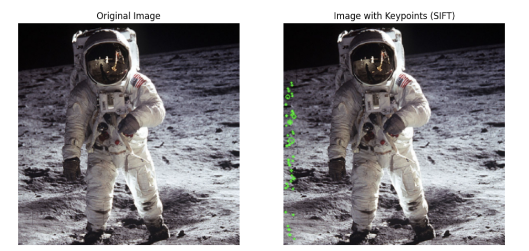
Detecting Keypoints using FAST (Features from Accelerated Segment Test)
FAST detects corners in an image by analyzing pixel intensities in a circular pattern around a candidate pixel. If a sufficient number of contiguous pixels in the circle are either brighter or darker than the central pixel, the central pixel is marked as a corner. FAST is one of the fastest detectors and works well when only corners are needed as keypoints. However, it lacks scale and orientation invariance by itself.
# Load an image in color
img = cv2.imread('astro.jpg')

# Convert the image to grayscale
gray = cv2.cvtColor(img, cv2.COLOR_BGR2GRAY)

# Step 1: Initialize the FAST detector
fast = cv2.FastFeatureDetector_create()

# Step 2: Detect keypoints
keypoints = fast.detect(gray, None)

# Step 3: Draw only a subset of keypoints (e.g., first 50 keypoints)
keypoints_subset = keypoints[:50]  # Take the first 50 keypoints

# Draw the selected keypoints on the original image
img_with_keypoints = cv2.drawKeypoints(img, keypoints_subset, None, color=(0, 255, 0), flags=cv2.DrawMatchesFlags_DRAW_RICH_KEYPOINTS)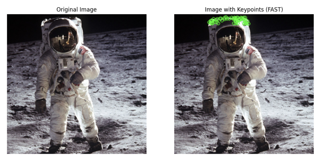
Detecting Keypoints using ORB (Oriented FAST and Rotated BRIEF)
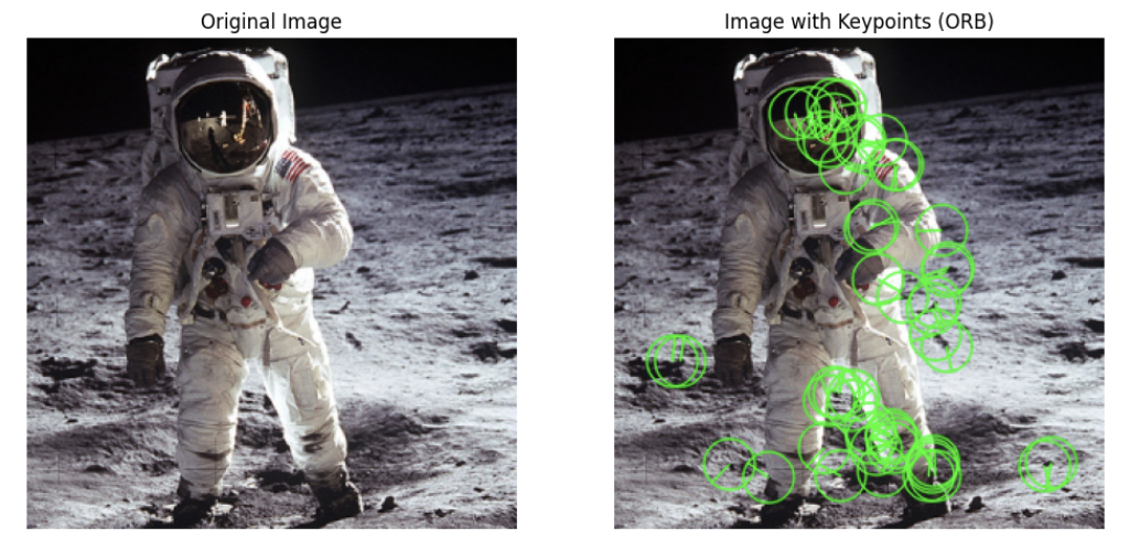
ORB is a feature (keypoint) detection and description algorithm that combines the FAST keypoint detector and BRIEF descriptor with several modifications to enhance performance. It uses FAST to detect keypoints and then applies the Harris corner measure to retain only the top N keypoints.
To handle images at different scales, ORB uses an image pyramid to detect features across multiple levels. A key limitation of FAST is its lack of rotation invariance, which ORB overcomes by calculating the orientation of each keypoint. This is done by finding the intensity-weighted centroid of the patch around the keypoint and using the direction from the keypoint to the centroid to assign orientation.
Here is the example of how to detect the keypoints in an image and display it.
# Load an image in color
img = cv2.imread('astro.jpg')

# Convert the image to grayscale
gray = cv2.cvtColor(img, cv2.COLOR_BGR2GRAY)

# Step 1: Initialize the ORB detector
orb = cv2.ORB_create()

# Step 2: Detect keypoints
keypoints = orb.detect(gray, None)

# Step 3: Draw only a subset of keypoints (e.g., first 50 keypoints)
keypoints_subset = keypoints[:50]  # Take the first 50 keypoints

# Draw the selected keypoints on the original image
img_with_keypoints = cv2.drawKeypoints(img, keypoints_subset, None, color=(0, 255, 0), flags=cv2.DrawMatchesFlags_DRAW_RICH_KEYPOINTS)
The code generates following output.
Computing Descriptors
After detecting keypoints, a descriptor is computed for each keypoint. A descriptor is a mathematical representation (usually a vector) that describe the local appearance around each keypoint in an image. Descriptors are computed after detecting keypoints and encode information about the surrounding pixel intensities or patterns in a way that is robust to various transformations such as scale, rotation, and illumination changes.
While keypoints tell us "where" the interesting points in an image are, descriptors help us understand "what" these points look like. Descriptors are crucial for comparing keypoints across different images, which allows us to match corresponding features. It help in following:
- Summarize Local Image Information: Descriptors encode information about the appearance of the pixels around a keypoint in a compact vector or binary string.
- Allow Keypoint Comparison: Descriptors allow us to numerically compare keypoints across images using distance metrics like the Euclidean distance or Hamming distance.
Here, we learn how to compute descriptors using SIFT and ORB.
Computing Descriptor using SIFT
SIFT calculates descriptors by analyzing the local gradients (changes in pixel intensities) around each keypoint. A 16x16 patch of pixels around the keypoint is divided into 4x4 subregions, and for each subregion, a histogram of 8 gradient orientations is created. This results in 16 histograms with 8 bins each, producing a 128-dimensional descriptor.
The descriptor is then normalized to enhance robustness against lighting and contrast changes. By capturing the distribution of local gradients, the SIFT descriptor is invariant to scale, rotation, and illumination, making it effective for matching keypoints across transformed images.
# Load an image
img = cv2.imread('astro.jpg')

# Convert the image to grayscale (SIFT works on grayscale images)
gray = cv2.cvtColor(img, cv2.COLOR_BGR2GRAY)

# Step 1: Initialize the SIFT detector
sift = cv2.SIFT_create()

# Step 2: Detect keypoints and compute descriptors
keypoints, descriptors = sift.detectAndCompute(gray, None)

# Step 3: Select two specific keypoints (first two keypoints as an example)
keypoints_subset = keypoints[:2]  # Take the first two keypoints
descriptors_subset = descriptors[:2]  # Take the corresponding descriptors

# Step 4: Draw the two selected keypoints on the original image
img_with_keypoints = cv2.drawKeypoints(img, keypoints_subset, None, color=(0, 255, 0), flags=cv2.DrawMatchesFlags_DRAW_RICH_KEYPOINTS)
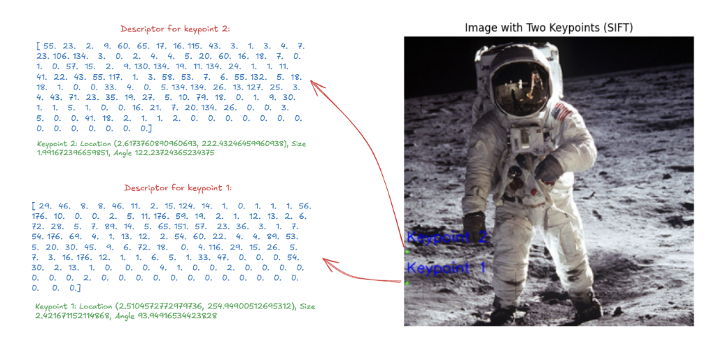
Here, we calculate two descriptor for the two keypoints as shown in image below.
Computing Descriptor using ORB (Oriented FAST and Rotated BRIEF)
ORB uses BRIEF descriptors for keypoints, but since BRIEF doesn't work well with rotation, ORB adjusts (or "steers") the BRIEF descriptors to match the orientation of the keypoints.
When a keypoint’s orientation is calculated, ORB rotates the BRIEF pattern (a set of binary comparisons between pixel pairs) by the same angle, ensuring that the descriptor is aligned with the keypoint's rotation. ORB breaks the rotation angle into small increments (12 degrees) and precomputes rotated BRIEF patterns for efficiency.
A good descriptor needs to be discriminative, meaning it should be able to distinguish between different features. BRIEF is effective because each of its binary comparisons (bits) has high variability and a mean value near 0.5, making it more likely to differentiate between different keypoints.
However, when BRIEF is rotated, it loses some of these qualities. To maintain high discrimination, ORB searches through possible binary tests to select those that maintain high variance, have a mean close to 0.5, and are uncorrelated. This improved version of BRIEF in ORB is called rBRIEF, which is more robust to rotation and ensures reliable feature matching.
Here’s an example where we detect first two keypoints and compute their descriptors using ORB:
# Convert the image to grayscale (ORB works on grayscale images)
gray = cv2.cvtColor(img, cv2.COLOR_BGR2GRAY)

# Step 1: Initialize the ORB detector
orb = cv2.ORB_create()

# Step 2: Detect keypoints and compute descriptors
keypoints, descriptors = orb.detectAndCompute(gray, None)

# Step 3: Select two specific keypoints (first two keypoints as an example)
keypoints_subset = keypoints[:2]  # Take the first two keypoints
descriptors_subset = descriptors[:2]  # Take the corresponding descriptors

# Step 4: Draw the two selected keypoints on the original image
img_with_keypoints = cv2.drawKeypoints(img, keypoints_subset, None, color=(0, 255, 0), flags=cv2.DrawMatchesFlags_DRAW_RICH_KEYPOINTS)

# Step 5: Add labels to the keypoints on the image
# Loop over each keypoint and add a label at its location
for i, keypoint in enumerate(keypoints_subset):
    x, y = int(keypoint.pt[0]), int(keypoint.pt[1])  # Get the keypoint coordinates
    label = f"Keypoint {i + 1}"  # Create a label for each keypoint
    cv2.putText(img_with_keypoints, label, (x, y - 10), cv2.FONT_HERSHEY_SIMPLEX, 0.5, (255, 0, 0), 1, cv2.LINE_AA)
The code will generate following output image with descriptors.

The descriptor in the image is a binary ORB descriptor for a specific keypoint (keypoint 1 and keypoint 2 in our example). This descriptor is a 32-element vector (in this case, 32 integers). Each of these 32 integers represents 8 bits of binary information that encodes the result of pixel intensity comparisons around the keypoint. This is how ORB summarizes the local patch around the keypoint into a compact binary form.
Matching Descriptors
Once keypoints and descriptors are extracted from two images, feature matching is performed by comparing the descriptors. Common methods to compare descriptors include:
Matching Descriptors using Brute-Force Matching
Brute-Force Matching method compares each descriptor in one image with every descriptor in the other image.
A distance metric (like Euclidean distance for float descriptors like SIFT descriptor or Hamming distance for binary descriptors like ORB descriptor, BRIEF) is used to measure the similarity between descriptors. Brute-force matching is straightforward and reliable but computationally expensive, especially for large images or a high number of keypoints. It Compares each descriptor in image 1 with all descriptors in image 2 and finds the single best match based on distance. In OpenCV, BFMatcher.match() returns the best match for each descriptor.
# Load two images
img1 = cv2.imread('object.jpg', cv2.IMREAD_GRAYSCALE)  # First image
img2 = cv2.imread('scene.jpg', cv2.IMREAD_GRAYSCALE)  # Second image

# Step 1: Initialize the ORB detector
orb = cv2.ORB_create()

# Step 2: Detect keypoints and compute descriptors for both images
keypoints1, descriptors1 = orb.detectAndCompute(img1, None)
keypoints2, descriptors2 = orb.detectAndCompute(img2, None)

# Step 3: Use BFMatcher (Brute-Force Matcher) to match descriptors
bf = cv2.BFMatcher(cv2.NORM_HAMMING, crossCheck=True)  # Hamming distance for ORB descriptors

# Step 4: Match descriptors between the two images
matches = bf.match(descriptors1, descriptors2)

# Step 5: Sort matches based on their distance (lower distance is better)
matches = sorted(matches, key=lambda x: x.distance)

# Step 6: Visualize the top 10 matches
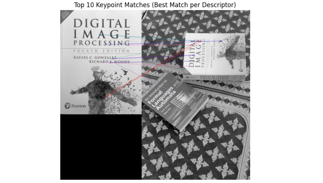
img_matches = cv2.drawMatches(img1, keypoints1, img2, keypoints2, matches[:10], None, flags=cv2.DrawMatchesFlags_NOT_DRAW_SINGLE_POINTS)
In this code the BFMatcher compares every descriptor in img1 with every descriptor in img2 using the Hamming distance. The Hamming distance measures how different the binary descriptors are. The lower the distance, the better the match. The crossCheck=True ensures mutual matching, meaning that a keypoint from image 1 matches with a keypoint from image 2 must also match back from image 2 to image 1. The top 10 matches (those with the smallest Hamming distances) are drawn with lines connecting the corresponding keypoints in both images using cv2.drawMatches().

The best match (the one with the smallest Hamming distance) is selected (in the image below). The coordinates of the matched keypoints in both images are printed for reference. The descriptors of these two keypoints are printed to show how they look.
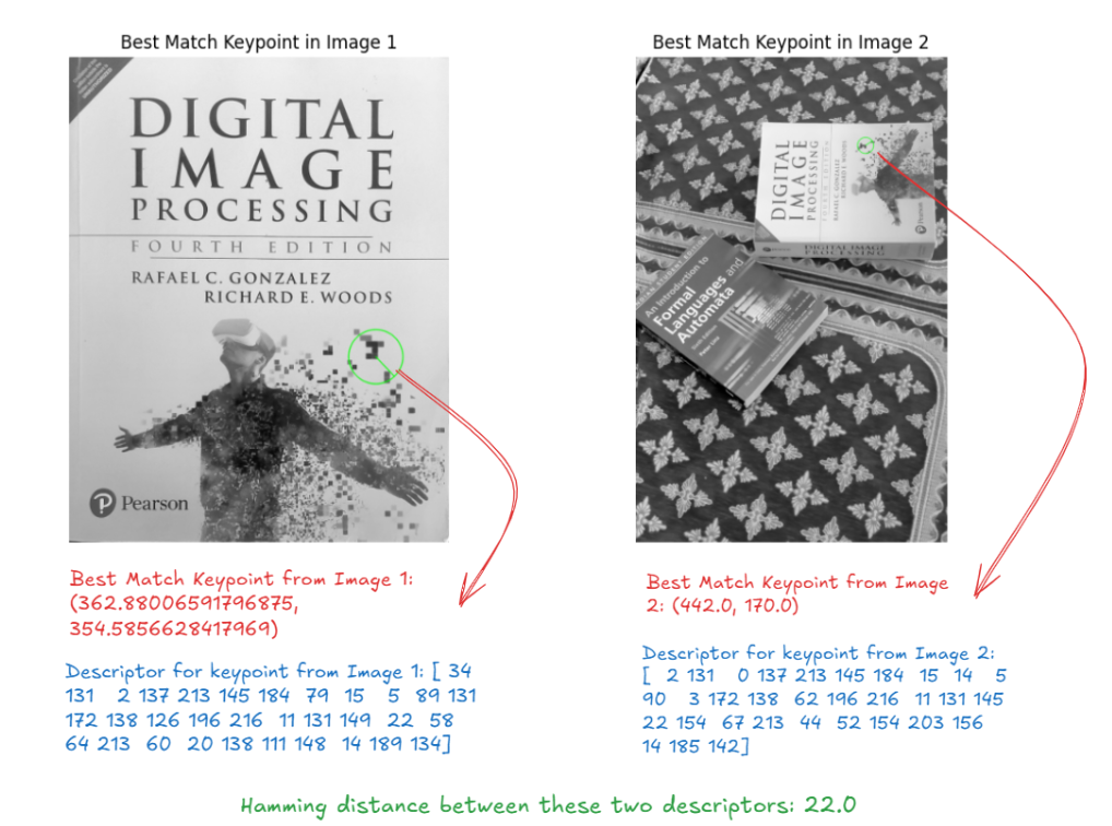
In the image above, the Hamming distance between the two descriptors is 22, meaning that 22 bits differ between the two 32-byte descriptors. This difference is used by BFMatcher to determine how similar or dissimilar two keypoints are. Lower distances represent better matches, while higher distances indicate more dissimilarity.
Matching Descriptors using KNN (K-Nearest Neighbors) for Brute-Force Matching
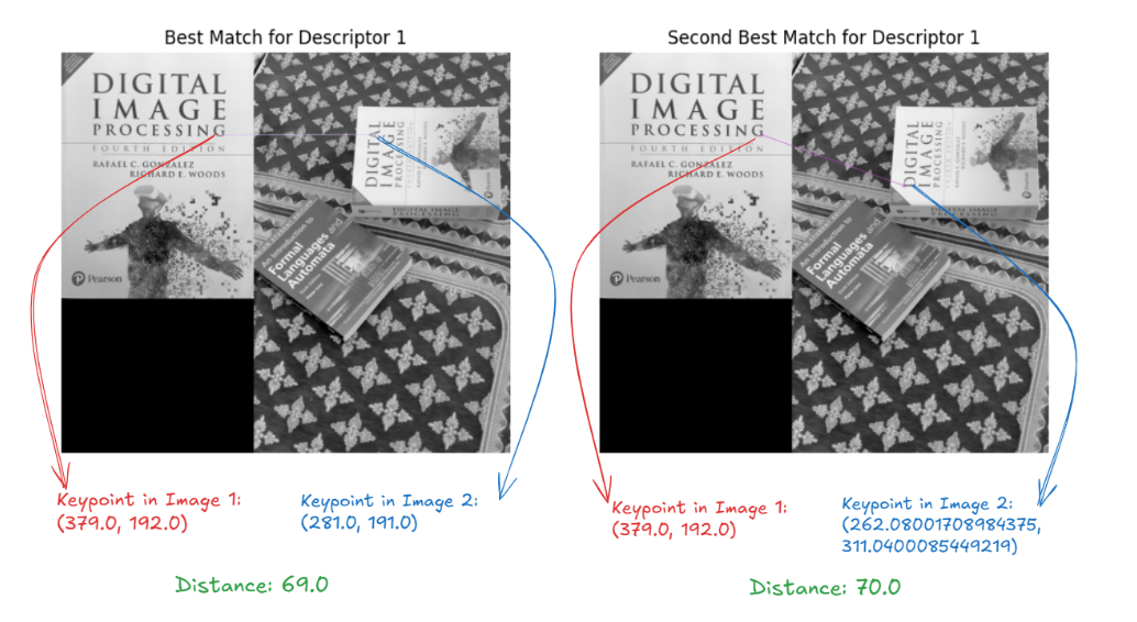
The Brute-Force matching also provides KNN matching via BFMatcher.knnMatch() to get k best matches. Here, instead of returning just the best match it returns k best matches for each descriptor. For each descriptor in the first image, KNN finds the top K nearest descriptors from the second image. K is usually set to 2, so that two nearest matches are retrieved. This allows us to apply filtering techniques like the Lowe’s ratio test (discussed below) to refine the matching and reduce incorrect matches. It compares each descriptor in image 1 with all descriptors in image 2 and finds the k best matches (k nearest neighbors) based on distance. In OpenCV BFMatcher.knnMatch() returns the k best matches for each descriptor. This means for each descriptor in the first image, you get k best matches in the second image.
KNN matching returns the k best matches for each descriptor. Following the definition, in the above example code we visualize the top 2 matches for first descriptor to illustrate this. In the image below, you can clearly see that same keypoint ([379.0, 192.0]) in the image 1 has two best matches ([281.0, 191.0] and [262.0, 311.0]) in the image 2.
Matching Descriptors using FLANN (Fast Library for Approximate Nearest Neighbors)
FLANN is an optimized algorithm designed to quickly find approximate nearest neighbors in large datasets. FLANN is used for fast feature matching. Instead of comparing every descriptor from one image to every descriptor from another (as brute-force matching does), FLANN uses efficient data structures like KD-Trees for floating-point descriptors and Locality Sensitive Hashing (LSH) for binary descriptors like ORB.
Matching Descriptors using Locality Sensitive Hashing (LSH)
LSH is a technique designed for binary descriptors, generated by ORB or BRIEF. It hashes similar data points into the same "buckets," ensuring that points that are close together in the original space have a high probability of being hashed into the same bucket. This makes it effective for fast nearest-neighbor searches in binary spaces, providing approximate but very efficient matching.
Here is the example code:
# Load two images that have some overlap
img1 = cv2.imread('object.jpg', cv2.IMREAD_GRAYSCALE)  # First image
img2 = cv2.imread('scene.jpg', cv2.IMREAD_GRAYSCALE)   # Second image

# Step 1: Initialize the ORB
orb = cv2.ORB_create()

# Step 2: Detect keypoints and compute descriptors for both images
keypoints1, descriptors1 = orb.detectAndCompute(img1, None)
keypoints2, descriptors2 = orb.detectAndCompute(img2, None)

# Step 3: Use FLANN-based matcher for ORB descriptors
FLANN_INDEX_LSH = 6
index_params = dict(algorithm=FLANN_INDEX_LSH, table_number=6, key_size=12, multi_probe_level=1)
search_params = dict(checks=50)

# Initialize FLANN-based matcher
flann = cv2.FlannBasedMatcher(index_params, search_params)

# Step 4: Match descriptors between the two images using KNN (k=2 for 2 nearest neighbors)
matches = flann.knnMatch(descriptors1, descriptors2, k=2)
The following output will be generated.
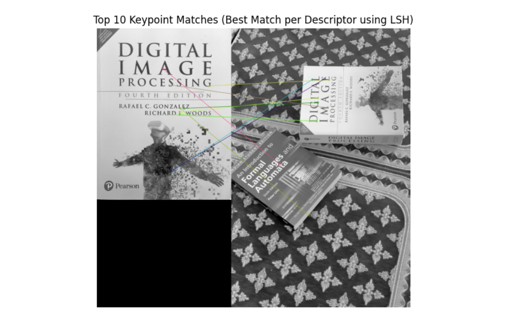
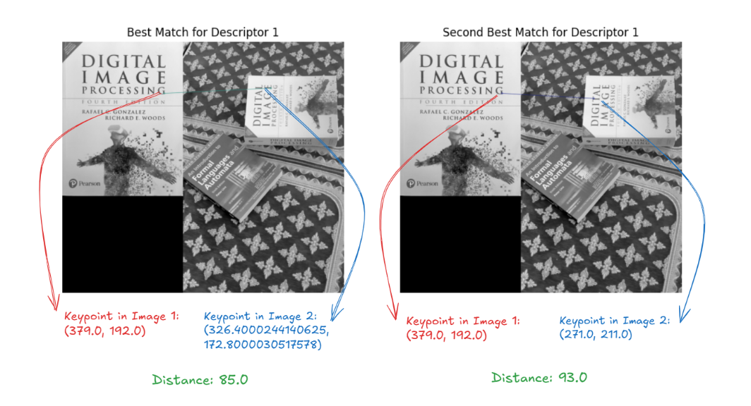
In this example we also visualize two matches for the first descriptor.
Matching Descriptors using KD-Tree (K-Dimensional Tree)
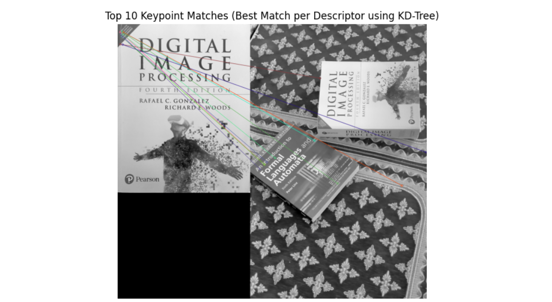
KD-Tree, on the other hand, is used for floating-point descriptors such as those from SIFT or SURF. It organizes data points in a tree structure based on their dimensions (k-dimensions) to allow efficient search for the nearest neighbors.
Here is the example code:
# Load two images
img1 = cv2.imread('object.jpg', cv2.IMREAD_GRAYSCALE)  # First image
img2 = cv2.imread('scene.jpg', cv2.IMREAD_GRAYSCALE)   # Second image

# Step 1: Initialize the SIFT detector (for KD-Tree, we use SIFT)
sift = cv2.SIFT_create()

# Step 2: Detect keypoints and compute descriptors for both images
keypoints1, descriptors1 = sift.detectAndCompute(img1, None)
keypoints2, descriptors2 = sift.detectAndCompute(img2, None)

# Step 3: Use FLANN-based matcher for SIFT descriptors (KD-Tree)
FLANN_INDEX_KDTREE = 1  # KD-Tree for SIFT (floating-point descriptors)
index_params = dict(algorithm=FLANN_INDEX_KDTREE, trees=5)  # Parameters for KD-Tree
search_params = dict(checks=50)  # Number of recursive checks in the tree

# Initialize FLANN-based matcher
flann = cv2.FlannBasedMatcher(index_params, search_params)

# Step 4: Match descriptors between the two images using KNN (k=2 for 2 nearest neighbors)
matches = flann.knnMatch(descriptors1, descriptors2, k=2)
The following will be the output generated by code:
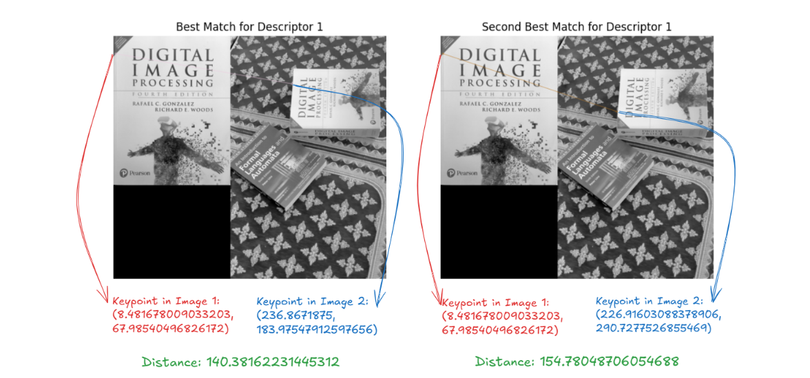
Here also, we visualize two matches for the first descriptor:
Filtering Matches
Feature matching often produces many incorrect or weak matches. To remove false positives and improve the accuracy of matching a filtering method is applied as discussed below.
Lowe’s Ratio Test
When KNN is used to find the two nearest matches for each keypoint, the ratio between the distances of the best match and the second-best match is calculated. If the ratio is below a certain threshold (e.g. 0.5), the match is considered reliable. If the ratio is above the threshold, the match is rejected. This technique helps eliminate ambiguous matches, especially in cases where multiple keypoints may have similar descriptors.
Here’s an example where apply Lowe's Ratio Test to filter good matches. Lowe's Ratio Test is a technique used to filter out ambiguous or false matches when performing feature matching. The idea is that for each keypoint in the first image, we consider the two best matches in the second image and apply the ratio test. The ratio test compares the distance of the closest match to the second-closest match, and if the ratio is below a certain threshold (typically 0.5), we accept the match as valid.
# Load two images
img1 = cv2.imread('object.jpg', cv2.IMREAD_GRAYSCALE)  # First image
img2 = cv2.imread('scene.jpg', cv2.IMREAD_GRAYSCALE)  # Second image

# Step 1: Initialize the ORB detector
orb = cv2.ORB_create()

# Step 2: Detect keypoints and compute descriptors for both images
keypoints1, descriptors1 = orb.detectAndCompute(img1, None)
keypoints2, descriptors2 = orb.detectAndCompute(img2, None)

# Step 3: Initialize BFMatcher with Hamming distance
bf = cv2.BFMatcher(cv2.NORM_HAMMING)

# Step 4: Use knnMatch to find the two best matches for each descriptor
matches = bf.knnMatch(descriptors1, descriptors2, k=2)  # k=2 to get the two best matches

# Step 5a: Without Lowe's Ratio Test, simply take the first match for each keypoint
matches_without_ratio = [m[0] for m in matches]  # Take the best match from each pair

# Step 5b: Apply Lowe's Ratio Test to filter out ambiguous matches
matches_with_ratio = []
for m, n in matches:
    if m.distance < 0.5 * n.distance:  # Lowe's ratio test
        matches_with_ratio.append(m)

# Step 6: Draw the matches for both approaches
img_matches_without_ratio = cv2.drawMatches(img1, keypoints1, img2, keypoints2, matches_without_ratio[:10], None, flags=cv2.DrawMatchesFlags_NOT_DRAW_SINGLE_POINTS)
img_matches_with_ratio = cv2.drawMatches(img1, keypoints1, img2, keypoints2, matches_with_ratio[:10], None, flags=cv2.DrawMatchesFlags_NOT_DRAW_SINGLE_POINTS)

Feature Matching Use Case
Feature matching enables object recognition by identifying keypoints in both the object and the scene, allowing for accurate detection even when the object is rotated, scaled, or partially occluded.
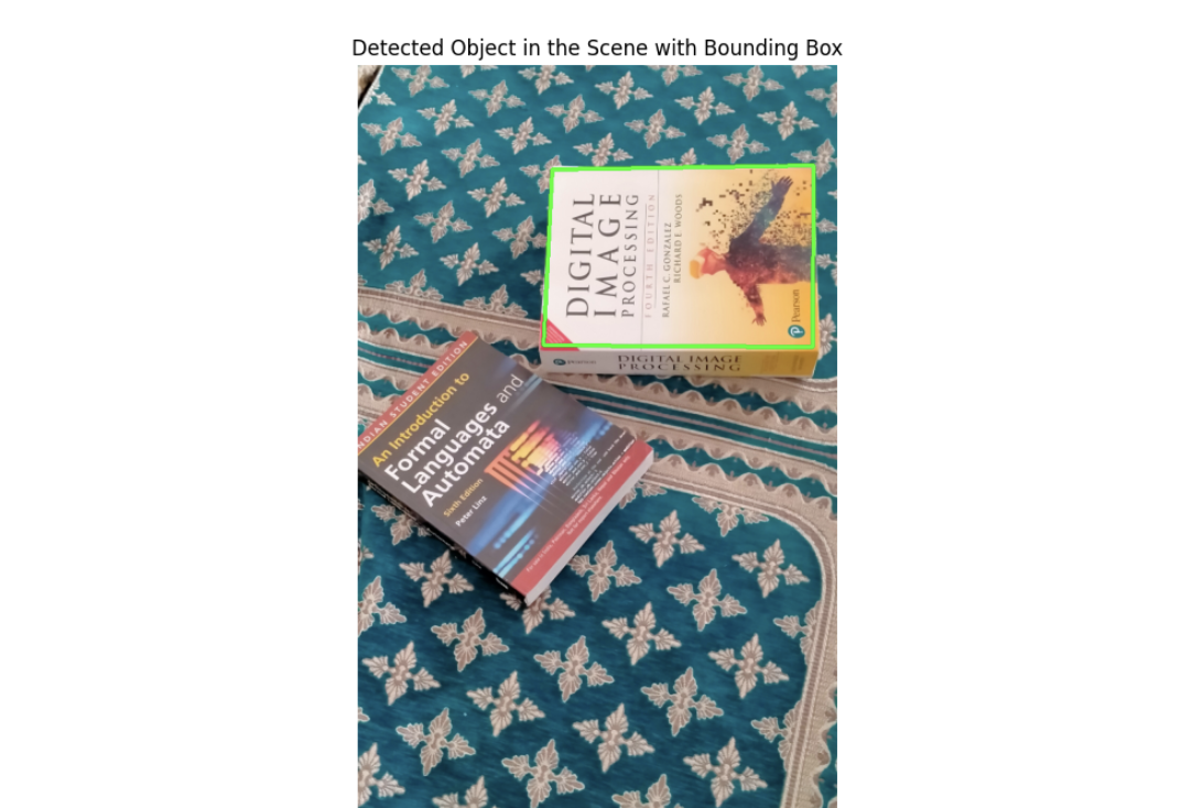
In this example, we'll use ORB for feature detection and matching to recognize an object (template) in a larger scene (image). The example demonstrates how feature matching can be used for object recognition, and how the detected object can be highlighted with a bounding box in the scene.
We draw a bounding box around the detected object in the scene, using the homography matrix to identify the object's location. The bounding box will be drawn using the corners of the object image, and we will map those corners onto the scene.
# Step 1: Load the object image (template) and the scene image
object_image = cv2.imread('object.jpg', cv2.IMREAD_GRAYSCALE)  # The object we want to recognize
scene_image = cv2.imread('scene.jpg', cv2.IMREAD_GRAYSCALE)  # The scene where we want to find the object

# Step 2: Initialize ORB detector
orb = cv2.ORB_create()

# Step 3: Detect keypoints and compute descriptors for both the object and scene
keypoints_obj, descriptors_obj = orb.detectAndCompute(object_image, None)
keypoints_scene, descriptors_scene = orb.detectAndCompute(scene_image, None)

# Step 4: Initialize BFMatcher and match descriptors
bf = cv2.BFMatcher(cv2.NORM_HAMMING, crossCheck=True)
matches = bf.match(descriptors_obj, descriptors_scene)

# Sort matches by distance (lower distance = better match)
matches = sorted(matches, key=lambda x: x.distance)

# Step 5: Visualize the top 10 matches between the object and the scene
matched_image = cv2.drawMatches(object_image, keypoints_obj, scene_image, keypoints_scene, matches[:10], None, flags=cv2.DrawMatchesFlags_NOT_DRAW_SINGLE_POINTS)

plt.figure(figsize=(15, 8))
plt.imshow(matched_image)
plt.title('Top 10 Feature Matches Between Object and Scene')
plt.axis('off')
plt.show()

# Step 6: Extract the matching keypoints positions
obj_pts = np.float32([keypoints_obj[m.queryIdx].pt for m in matches]).reshape(-1, 1, 2)
scene_pts = np.float32([keypoints_scene[m.trainIdx].pt for m in matches]).reshape(-1, 1, 2)

# Step 7: Find the homography matrix to map the object image to the scene
H, mask = cv2.findHomography(obj_pts, scene_pts, cv2.RANSAC, 5.0)

# Step 8: Get the dimensions of the object image
h, w = object_image.shape

# Step 9: Define the object image corners and transform them to the scene using the homography
object_corners = np.float32([[0, 0], [0, h], [w, h], [w, 0]]).reshape(-1, 1, 2)
scene_corners = cv2.perspectiveTransform(object_corners, H)

# Step 10: Load the original scene image in color
scene_image_color = cv2.imread('scene.jpg')

# Step 11: Draw the detected object location in the scene image
cv2.polylines(scene_image_color, [np.int32(scene_corners)], True, (0, 255, 0), 3)  # Green bounding box
Conclusion
In this blog post we have explored feature matching, understanding how it works. Feature matching is used in many computer vision applications, such as object recognition, image stitching, 3D reconstruction, image matching and object tracking. Using Roboflow’s no-code approach, you can implement feature matching, by applying the Scale-Invariant Feature Transform (SIFT) method.
All the code for this blog post is available in this notebook.
Cite this Post
Use the following entry to cite this post in your research:
Timothy M. (Oct 30, 2024). What is Feature Matching?. Roboflow Blog: https://blog.roboflow.com/what-is-feature-matching/
