
In this blog post, we will explore some commonly used methods for hyperparameter tuning, including manual hyperparameter tuning, grid search, random search, and Bayesian optimization.
Hyperparameter Tuning
Machine learning involves understanding the relationship between independent and dependent variables. When working on machine learning projects, a considerable amount of time is dedicated to tasks like Exploratory Data Analysis and feature engineering. Another crucial aspect of model development is hyperparameter tuning.
Hyperparameter tuning focuses on fine-tuning the hyperparameters to enable the machine to construct a robust model that performs well on unseen data. Effective hyperparameter tuning, in addition to quality feature engineering, can significantly enhance the performance of the model. While many advanced machine learning models like Bagging (Random Forests) and Boosting (XGBoost, LightGBM, etc.) are already optimized with default hyperparameters, there are instances where manual tuning can lead to better model outcomes.
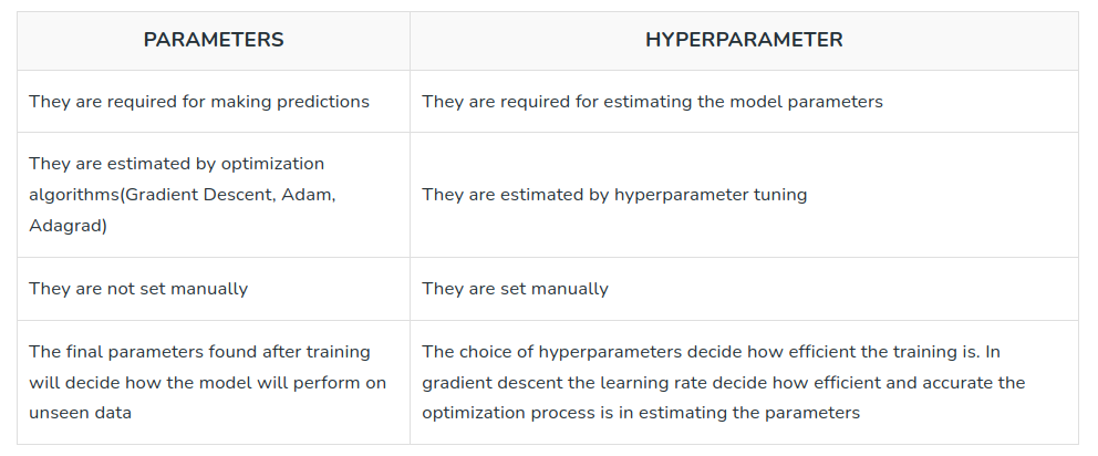
Parameters vs Hyperparameters
Understanding the distinction between parameters and hyperparameters is crucial in machine learning. Let's delve into the key differences between these two concepts.
What is a Parameter in Machine Learning?
Parameters in machine learning models are the variables that the model learns from the available data during the training process. They directly affect the model's performance and represent the internal state or characteristics of the model. Parameters are typically optimized by adjusting their values through an optimization algorithm like gradient descent.
For example, in a linear regression model, the parameters are the coefficients associated with each input feature. The model learns these coefficients based on the provided data, aiming to find the best values that minimize the difference between the predicted output and the actual output.
In Convolutional Neural Networks (CNNs), the parameters consist of the weights and biases associated with the network's layers. During training, these parameters are iteratively adjusted using backpropagation and optimization algorithms such as stochastic gradient descent.
In short, parameters are internal to the model and are learned from the data during training.
What is a Hyperparameter?
Hyperparameters define the configuration or settings of the model. They are not learned from the data, but instead we provide them as inputs before training the model. Hyperparameters guide the learning process and impact how the model behaves during training and prediction.
Hyperparameters are set by machine learning engineer(s) and/or researcher(s) working on a project based on their expertise and domain knowledge. Tuning these hyperparameters is essential for improving the model's performance and generalization ability.
Examples of hyperparameters in computer vision include the learning rate, batch size, number of layers, filter sizes, pooling strategies, dropout rates, and activation functions. These hyperparameters are set based on specific characteristics of the dataset, the complexity of the task, and the available computational resources.
Fine-tuning hyperparameters can have a significant impact on the model's performance in computer vision tasks. For example, adjusting the learning rate can affect the convergence speed and prevent the model from getting stuck in suboptimal solutions. Similarly, tuning the number of layers and filter sizes in a CNN can determine the model's ability to capture intricate visual patterns and features.
The table below summarizes the difference between model parameters and hyperparameters.
Common Hyperparameters in Computer Vision
In computer vision tasks, various hyperparameters significantly impact the performance and behavior of machine learning models. Understanding and appropriately tuning these hyperparameters can greatly enhance the accuracy and effectiveness of computer vision applications. Here are some common hyperparameters encountered in computer vision:
- Learning Rate: The learning rate determines the step size at which the model updates its parameters during training. It influences the convergence speed and stability of the training process. Finding an optimal learning rate is crucial to prevent underfitting or overfitting.
- Batch Size: The batch size determines the number of samples processed in each iteration during model training. It affects the training dynamics, memory requirements, and generalization ability of the model. Choosing an appropriate batch size depends on the available computational resources and characteristics of the dataset on which the model will be trained.
- Network Architecture: The network architecture defines the structure and connectivity of neural network layers. It includes the number of layers, the type of layers (convolutional, pooling, fully connected, etc.), and their configuration. Selecting an appropriate network architecture depends on the complexity of the task and the available computational resources.
- Kernel Size: In convolutional neural networks (CNNs), the kernel size determines the receptive field size used for feature extraction. It affects the level of detail and spatial information captured by the model. Tuning the kernel size is essential to balance local and global feature representation.
- Dropout Rate: Dropout is a regularization technique that randomly drops a fraction of the neural network units during training. The dropout rate determines the probability of “dropping” each unit. Dropout rate helps prevent overfitting by encouraging the model to learn more robust features and reduces the dependence on specific units.
- Activation Functions: Activation functions introduce non-linearity to the model and determine the output of a neural network node. Common activation functions include ReLU (Rectified Linear Unit), sigmoid, and tanh. Choosing an appropriate activation function can impact the model's capacity to capture complex relationships and its training stability.
- Data Augmentation: Data augmentation techniques, such as rotation, scaling, and flipping, enhance the diversity and variability of the training dataset. Hyperparameters related to data augmentation, such as rotation angle range, scaling factor range, and flipping probability, influence the augmentation process and can improve the model's ability to generalize to unseen data.
- Optimization Algorithm: The choice of optimization algorithm influences the model's convergence speed and stability during training. Common optimization algorithms include stochastic gradient descent (SGD), ADAM, and RMSprop. Hyperparameters related to the optimization algorithm, such as momentum, learning rate decay, and weight decay, can significantly impact the training process.
Tuning these hyperparameters requires careful experimentation and analysis to find the optimal values for a specific computer vision task. The trade-offs between computational resources, dataset characteristics, and model performance must be taken into account to achieve the best results.
How to Tune Hyperparameters
In this section, we will discuss common methods for tuning hyperparameters in machine learning. Let’s begin!
Manual Hyperparameter Tuning
Manual hyperparameter tuning is a method of adjusting the hyperparameters of a machine learning model through manual experimentation. It involves iteratively modifying the hyperparameters and evaluating the model's performance until satisfactory results are achieved. Although this can be a time-consuming process, manual tuning provides the flexibility to explore various hyperparameter combinations and adapt them to specific datasets and tasks.
For example, let's consider a support vector machine (SVM) model. Some of the hyperparameters that can be manually tuned include the choice of the kernel (linear, polynomial, radial basis function), the regularization parameter (C), and the kernel-specific parameters (such as the degree for a polynomial kernel or gamma for an RBF kernel). By experimenting with different values for these hyperparameters and evaluating the model's performance using appropriate metrics, the optimal combination that yields the best results for the specific problem can be determined.
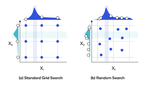
Hyperparameter Tuning with Grid Search
Grid search involves exhaustively searching a predefined set of hyperparameter values to find the combination that yields the best performance. A grid search systematically explores the hyperparameter space by creating a grid or a Cartesian product of all possible hyperparameter values and evaluating the model for each combination.
In grid search, it is required to define the range of values for each hyperparameter that needs to be tuned. The grid search algorithm then trains and evaluates the model using all possible combinations of these values. The performance metric, such as accuracy or mean squared error, is used to determine the best set of hyperparameters.
For example, consider a Random Forest classifier. The hyperparameters that can be tuned using grid search include the number of trees in the forest, the maximum depth of each tree, and the minimum number of samples required to split a node. By defining a grid of values for each hyperparameter, such as [100, 200, 300] for the number of trees and [5, 10, 15] for the maximum depth, grid search explores all possible combinations (e.g., 100 trees with a maximum depth of 5, 200 trees with a maximum depth of 10, etc.). The model is trained and evaluated for each combination, and the best-performing set of hyperparameters is selected.
Hyperparameter Tuning with Random Search
Unlike grid search, which exhaustively evaluates all possible combinations, random search randomly samples from a predefined distribution of hyperparameter values. This sampling process allows for more efficient and scalable exploration of the hyperparameter space.
In grid search, it is required to define the range of values for each hyperparameter that needs to be tuned. In contrast, using a random search the distribution or range of values is defined for each hyperparameter that needs to be tuned. The random search algorithm then samples combinations of hyperparameter values from these distributions and evaluates the model's performance. By iteratively sampling and evaluating a specified number of combinations, random search aims to identify the hyperparameter settings that yield the best performance.
For example, consider a gradient boosting machine (GBM) model. The hyperparameters that can be tuned using random search include the learning rate, the maximum depth of the trees, and the subsampling ratio.
Instead of specifying a grid of values, random search allows the engineer to define probability distributions for each hyperparameter. For instance, a uniform distribution for the learning rate between 0.01 and 0.1, a discrete distribution for the maximum depth between 3 and 10, and a normal distribution for the subsampling ratio centered around 0.8. The random search algorithm then randomly samples combinations of hyperparameters and evaluates the model's performance for each combination.
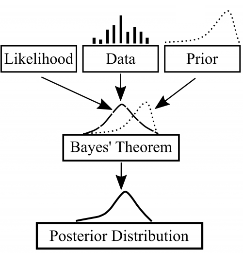
Hyperparameter Tuning with Bayesian Optimization
Bayesian optimization uses probabilistic models to efficiently search for the optimal hyperparameters. This works by sequentially evaluating a limited number of configurations based on their expected utility.
In Bayesian optimization, a probabilistic model, such as a Gaussian process, is built to approximate the objective function's behavior. This model is updated as new configurations are evaluated, capturing the relationships between hyperparameters and the corresponding performance. The model is then used to guide the search process and select the next set of hyperparameters to evaluate, aiming to maximize the objective function.
For example, consider a deep neural network model. Bayesian optimization can be employed to tune hyperparameters such as the learning rate, dropout rate, and number of hidden layers. The initial configurations are sampled randomly. As the surrogate model is updated, the algorithm intelligently selects new configurations to evaluate based on the expected improvement in performance. This iterative process allows Bayesian optimization to efficiently explore the hyperparameter space and identify the settings that yield the best model performance.
Hyperparameter Tuning with Bayesian Optimization in Computer Vision
Bayesian optimization is particularly beneficial in hyperparameter tuning for computer vision tasks. Here are a few examples of Bayesian optimization in computer vision:
- Image Style Transfer with Neural Networks: In image style transfer using neural networks, Bayesian optimization can be applied to tune hyperparameters such as the content weight, style weight, and the number of iterations. The model captures the relationship between hyperparameters and metrics like perceptual loss and style loss. Bayesian optimization guides the search process to identify hyperparameter settings that result in visually appealing stylized images.
- Image Recognition with Convolutional Neural Networks: Bayesian optimization can be used to tune hyperparameters for image recognition tasks using CNNs. Hyperparameters such as the learning rate, weight decay, and batch size can be optimized using this approach. The model captures the performance of the model in terms of accuracy, and Bayesian optimization intelligently explores the hyperparameter space to identify the combination that maximizes the recognition performance.
- Image Generation with Variational Autoencoders (VAEs): Bayesian optimization can be employed to tune hyperparameters in image generation tasks using VAEs. Hyperparameters such as the latent space dimension, learning rate, and batch size can be optimized. The model captures the reconstruction loss and generation quality, which can be used with Bayesian optimization to identify the hyperparameter settings that lead to better-quality generated images.
By leveraging probabilistic models and intelligent exploration, Bayesian optimization offers an effective approach for hyperparameter tuning in computer vision. It allows for efficient navigation of the hyperparameter space and helps identify optimal hyperparameter configurations, leading to improved performance and better outcomes in various computer vision tasks.
Hyperparameter Tuning Conclusion
Hyper parameter tuning is a crucial step in developing accurate and robust machine learning models. Manual tuning, grid search, random search, and Bayesian optimization are popular techniques for exploring the hyperparameter space.
Each method offers its own advantages and considerations. Machine learning practitioners work to find optimal configurations for a given model. Choosing the appropriate technique depends on factors such as search space size and computational resources.
In the field of computer vision, these techniques play a vital role in enhancing performance and achieving better outcomes.
By effectively employing these techniques, practitioners can optimize their models and unlock the full potential of their computer vision applications.
Cite this Post
Use the following entry to cite this post in your research:
Petru P.. (Jun 16, 2023). What is Hyperparameter Tuning? A Deep Dive. Roboflow Blog: https://blog.roboflow.com/what-is-hyperparameter-tuning/