Crack Detection with Computer Vision

Crack detection is the process of automatically identifying and analyzing cracks in structures, materials, or surfaces, which can be done using computer vision techniques.

Recent advances in deep learning have significantly improved the automation of crack detection across various domains. Traditional image processing methods often struggle with variations in lighting, texture, and complex backgrounds, whereas convolutional neural networks and modern architectures can learn discriminative features directly from data.

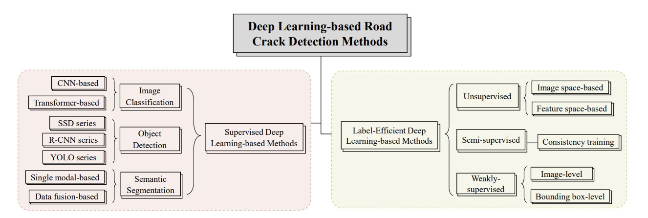
Computer vision techniques such as image classification, object detection, and segmentation techniques can help identify cracks with high accuracy, robustness, and scalability. These methods enable real-time, objective, and large-scale monitoring which makes them particularly valuable for safety-critical applications such as civil infrastructure, manufacturing, and quality control.

For example, in the paper Vehicular Road Crack Detection with Deep Learning, a road-mounted vehicular vision system is proposed where cameras capture pavement surfaces in real time as vehicles move.

These images are processed through deep learning pipelines implementing three approaches: 

• Classification models to simply flag whether a road segment has cracks or not.
• Object detection models (e.g., YOLO variants, RF-DETR) to locate and box cracked regions for easier indexing.
• Semantic segmentation models (e.g., U-Net, DeepLab) to provide pixel-wise maps of cracks, enabling measurement of crack length and width.

The system demonstrated that while classification is useful for quick binary screening and detection is efficient for localizing damaged spots, segmentation gave the most detailed structural assessment, allowing for precise monitoring of crack progression on highways. This kind of setup shows how computer vision deep learning system can be deployed in a moving vehicle to automate large-scale road health inspections.

Computer Vision for Crack Detection: Use Case Examples

Cracks in materials and structures can be detected using different computer vision approaches, depending on the nature of the problem. Image classification can be applied when the task is to simply determine whether a surface contains cracks or not. Object detection extends this by not only identifying cracks, but also localizing them within bounding boxes, making it useful in production-line inspections. Instance and semantic segmentation go even further by delineating the exact shape, boundaries, and size of cracks at the pixel level, which is essential for structural health monitoring.

Selecting the computer vision techniques for crack detection largely depends upon the task you want to perform or result you want to achieve. Following are three use case example that highlights use of three main computer vision approaches:

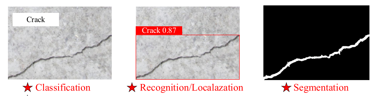
Use Case 1: Ceramic Tile Crack Detection (Image Classification)

In tile manufacturing, defects such as hairline cracks can compromise product quality and durability. By training a deep learning classification model (e.g., CNN, ResNet, ViT, MobileNet), ceramic tiles can be automatically categorized as “cracked” or “intact” using captured images. This ensures that defective tiles are quickly filtered out during quality control, reducing customer complaints and improving production efficiency.

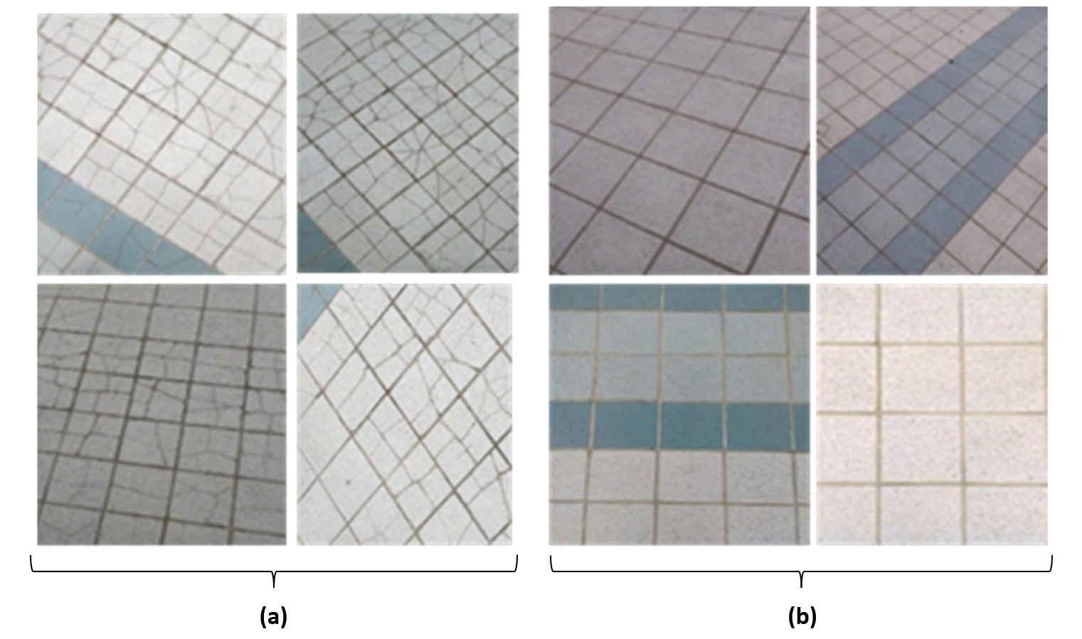
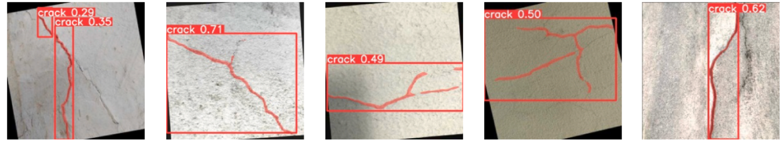
Use Case 2: Road Crack Detection (Object Detection)

Road pavements often develop cracks due to traffic loads, weathering, and aging, which, if left unmonitored, can lead to severe structural damage and costly repairs. Computer vision systems equipped with object detection models such as RF-DETR or YOLO can automatically scan road images captured by vehicle-mounted or drone-mounted cameras.

These models draw bounding boxes around cracked regions and enable engineers to localize and document defects across large pavement networks in real time. Automating this process, transportation authorities can quickly prioritize maintenance, reduce manual inspection effort, and improve road safety and longevity.

Use Case 3: Structural Monitoring on Concrete Surfaces (Segmentation)

Cracks in concrete structures such as building walls, bridges, and pavement are critical indicators of weakening integrity and potential failure. Advanced instance and semantic segmentation models (e.g., U-Net, DeepCrack, Mask R-CNN) generate pixel-level crack maps that not only highlight the exact shape and location of damage, but also enable precise measurement of crack length and width through skeletonization and distance mapping techniques.

By quantifying these parameters, engineers can better evaluate crack severity, track how defects propagate over time, and prioritize interventions. This detailed level of analysis makes segmentation especially valuable for proactive maintenance and long-term structural health monitoring.

From tile inspection in factories to large road networks and large-scale infrastructure monitoring, computer vision enables highly accurate and automated crack detection workflows. With the help of these computer vision techniques (e.g. classification, detection, and segmentation), industries and organizations can improve product quality, enhance safety, and reduce costs by replacing subjective human inspection with robust AI based systems.

Best Crack Detection Tools

When building a crack detection system, specialized platforms can save significant time in dataset preparation, training, and deployment. Roboflow is one of the most popular tools, offering end-to-end support for computer vision workflows with following key features:

• Simplifies dataset handling by allowing quick upload and annotation of crack images, with smart tools like Label Assist and Smart Polygon to accelerate labeling.
• Supports different workflows by enabling training for classification (cracked vs intact), object detection (bounding boxes around defects), and segmentation (pixel-level crack maps).
• Enhances model robustness with built-in tools for preprocessing (e.g., resizing, orientation, grayscale etc.) and augmentations (e.g. brightness, noise, and rotation etc.) helping models perform reliably under different lighting, textures, and environmental conditions.
• Provides a seamless pipeline for training deep learning models and deploying them to cloud, edge, or mobile devices for real-time crack detection.
• Offers clear metrics and visual dashboards to assess model accuracy, compare approaches, and continuously refine detection performance.

With these important capabilities, Roboflow enables researchers and engineers to handle different types of cracks across diverse domains, from tiny hairline fractures in ceramics to large surface cracks in pavements, using the most appropriate detection technique for the task.

Tutorial: How to do Crack Detection with Roboflow

Now let’s explore how crack detection can be implemented using Roboflow. In this section, we will cover how different computer vision approaches can be applied to the task, focusing on: 

• Object detection to identify and localize cracks with bounding boxes.
• Instance segmentation to generate pixel-level masks to capture the exact shape and size of cracks.

Before trying the example install the required libraries with following command:

pip install inference-sdk flet

Example #1: Crack detection using object detection

In this example, we build a crack detection system using Roboflow and build a Flet app for real-time crack inspection.

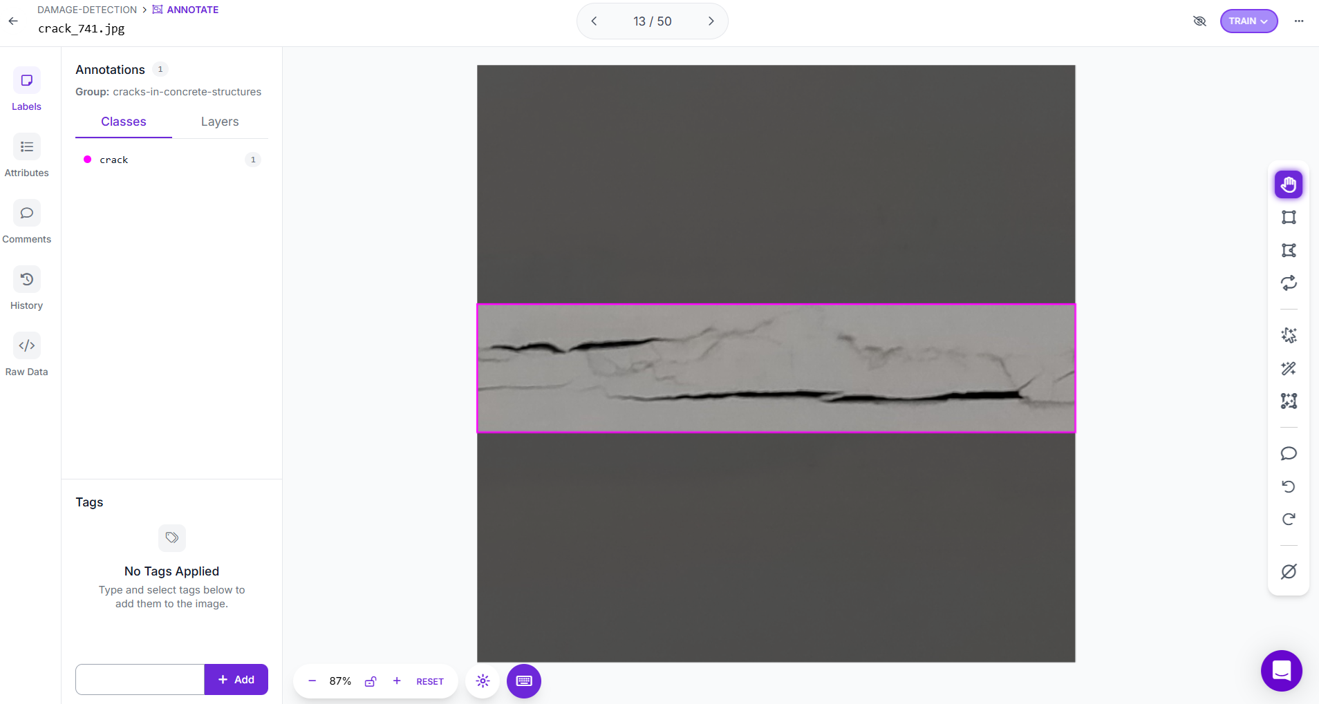
Step #1. Prepare a Dataset for Object Detection

The first step in building a crack detection system with Roboflow is to set up a new Object Detection project. Upload images that contain cracks on the surfaces you want to monitor, such as concrete, asphalt, or ceramic tiles. Using the annotation tools, draw bounding boxes tightly around each visible crack. Give each box the label “crack”, or, if you want to study different categories, create multiple labels such as hairline crack, wide crack, or surface fracture. Precision in annotation is important, boxes should include the entire crack while avoiding large amounts of background. Accurate labeling ensures that the model learns the right features during training.

Once annotation is complete, you can prepare dataset versions inside Roboflow. These versions may include preprocessing and augmentation to make the model robust under varied lighting and viewing conditions. Roboflow also helps split the dataset into training, validation, and test sets, ensuring balanced evaluation. Each version keeps your original annotations intact, so you can experiment with different preprocessing and augmentation strategies, train multiple models, and compare performance to select the best crack detection pipeline.

Step #2. Train Object Detection Model

Once the dataset is ready, the next step is to train a crack detection model using Roboflow Train. Training begins by selecting a model architecture. Options include RF-DETR, Roboflow 3.0, YOLOv11, and others, each with different trade-offs. For this project, I selected Roboflow 3.0.

The next step is choosing a model size. Roboflow provides options such as Fase, Accurate, Medium, Large and Extra Large. I selected the Accurate size.

Finally, Roboflow offers several training strategies:

• Train from Previous Checkpoint to continue improving an already trained model.
• Train from Public Checkpoint to start with pretrained weights from large datasets (e.g., COCO), then fine-tune for cracks.
• Train from Random Initialization to start from scratch (not recommended, as it needs more data and produces weaker results).

For this project, I chose Train from Public Checkpoint (MS COCO), which leverages pre-trained weights from a large benchmark dataset.

After confirming the configuration, clicking Start Training launches the training process  and after training is completed a crack detection model is ready for evaluation and real-world use.

Step #3. Build the Roboflow Workflow

Next, create a crack detection workflow in Roboflow to connect the trained model with visualization and output blocks.

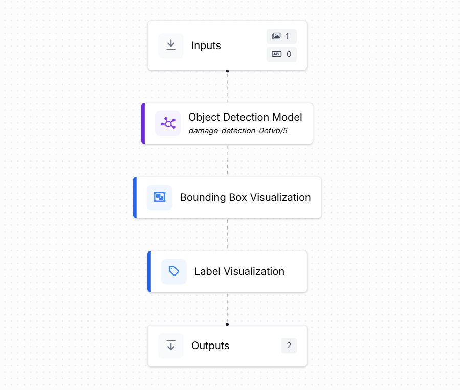
This workflow takes an input image, processes it through the trained crack object detection model, and produces both visual results (bounding boxes with labels) and structured outputs (coordinates and confidence scores). The workflow includes the following blocks:

• Inputs: Defines the incoming data to the workflow. In this case, the input is an image of a surface (e.g., concrete, pavement, tile) that may contain visible cracks.
• Object Detection Model: Uses the trained crack detection model (e.g., damage-detection-0otvb/5 in this case). The model predicts bounding boxes around each detected crack. For every bounding box, the model outputs structured prediction data, including:
  • Image width and height
  • Bounding box center coordinates (x, y)
  • Bounding box width and height
  • Prediction confidence score
• Bounding Box Visualization: Overlays the predicted bounding boxes directly onto the image, allowing visual verification of where cracks were detected.
• Label Visualization: Adds the crack class label (e.g., “crack”) together with the confidence score above each bounding box. This makes the output more interpretable for users.
• Outputs: Collects the final results. It produces:
  • Visual output - the image with bounding boxes and labels drawn on detected cracks.
  • Structured JSON output - containing image dimensions, bounding box coordinates, and confidence scores. This data can be used for further tasks such as defect reporting, statistical analysis, or integration with maintenance management systems.

In short, the workflow ingests an image, detects and localizes cracks with bounding boxes, provides an annotated image for quick inspection, and exports structured numerical predictions for downstream applications.

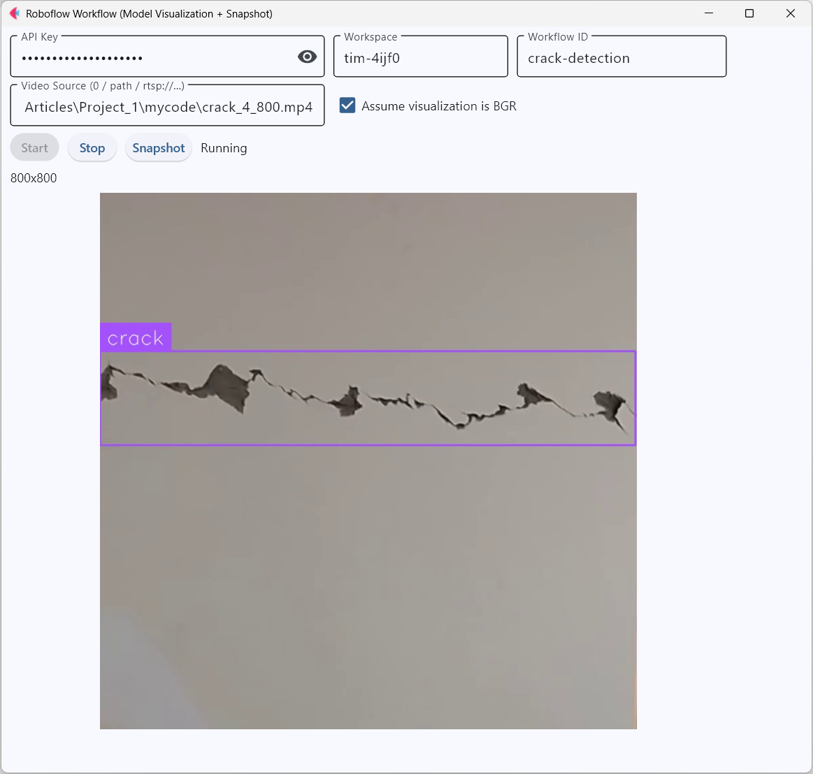
Step #4. Deploy the Roboflow Workflow

In this step, the trained crack detection workflow is deployed using a Flet app. The app connects to the Roboflow Workflow API and streams predictions from a camera feed or video source. For every frame, the app shows detection results with bounding boxes and labels drawn on the image. The interface includes controls to start/stop the pipeline, monitor the status, and capture snapshots of detected cracks for later review. This setup makes it possible to run real-time crack inspection from a simple desktop or web interface.

The code builds a Flet GUI application that runs your Roboflow workflow for crack detection:

• Interface controls: Text fields let you enter your API key, workspace, workflow ID, and video source (camera, file path, or RTSP stream). Buttons allow you to start, stop, and take snapshots.
• InferencePipeline: Connects to Roboflow’s hosted workflow and streams video frames through the trained model. Each frame is processed for crack detection.
• on_prediction() callback: Runs every time the model produces a result. It takes the detection output, overlays bounding boxes and labels on the image, and displays it in the app. The callback also enables the Snapshot button once predictions are available.
• Start/Stop logic: Uses a separate thread to run the detection pipeline so the app interface stays responsive.
• Snapshot feature: Saves the most recent detection frame (with bounding boxes) as a JPG file in a snapshots/ folder, using the current timestamp as the filename.
• Status updates: The app shows whether the pipeline is Idle, Starting, Running, or Stopped, making it clear what state the system is in.

In short, this code turns your trained crack detection model into a real-time inspection tool with a user-friendly interface, live visualization, and snapshot saving.

You can run the Flet App with following command for desktop version:

flet run app.py

You should see output similar to following.

Flet app can also be run in the web browser. Just add the --web option in command while executing.

flet run –-web app.py

and you should see output similar to following:

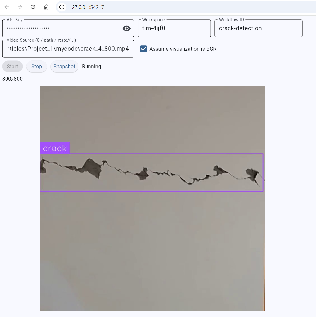
So, with the same code you will be able to run you application as standalone desktop application and a web application. Here I have used pre-recorded .mp4 file you may also try with you live camera/web cam or even rtsp.

Example #2: Crack detection using instance segmentation

In this example, we will build and use an instance segmentation model to detect cracks in images. The goal is to train the model to precisely map the shape, width, and length of cracks at the pixel level.

Step #1. Prepare a Dataset for Segmentation

For crack segmentation, begin by creating a Segmentation Project in Roboflow. After setting up the project, upload images. Using Roboflow’s polygon, carefully trace the exact outline of each crack. This allows the model to learn not just where cracks occur, but also their shape, continuity, and thickness.

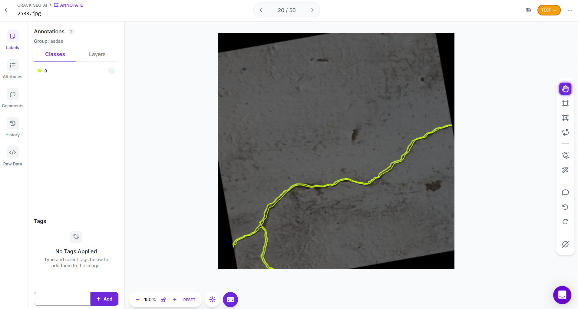
Each annotated region can be labeled as “crack.” If needed, you can define multiple classes to capture different types of cracks, such as hairline, wide etc. This makes the model capable of distinguishing between crack patterns, which is especially useful for monitoring structural severity. Roboflow’s Smart Polygon tool can speed up annotation by automatically snapping outlines to object boundaries.

Once annotation is complete, you can generate dataset versions with preprocessing (resizing, normalization) and augmentations such as rotation, blur, or brightness adjustments. These steps improve model robustness under different lighting or environmental conditions. Splitting the dataset into training, validation, and test sets ensures fair evaluation and prevents overfitting. 

Step #2. Train the Segmentation Model

Training a segmentation model in Roboflow Train starts with choosing a model architecture. Options include Roboflow 3.0 (YOLOv8-compatible with balanced speed and accuracy) or YOLOv11, optimized for fast inference. For this project, Roboflow 3.0 was selected, as it offers strong performance and smooth deployment.

Next, select the model size, which determines the trade-off between speed and accuracy. Options range from Nano (fastest, less accurate) to Extra Large (slowest, most accurate). For this task, a Medium model size was chosen to achieve higher accuracy while keeping training time manageable.

Finally, decide on the training strategy:

• Train from Previous Checkpoint -continue improving an already trained model.
• Train from Public Checkpoint - start with pretrained weights (e.g., MS COCO), leveraging prior knowledge of general shapes and textures.
• Train from Random Initialization - start from scratch (requires more data, not usually recommended).

For crack segmentation, training was initialized from a Public Checkpoint (MS COCO). This transfer learning approach allows the model to adapt quickly to crack-specific patterns while benefiting from prior general vision knowledge.

After confirming all settings, click Start Training to launch the training. Finally, you’ll have a deployable instance segmentation model capable of outlining cracks with high precision. 

Step #3. Build the Roboflow Workflow

Now we create a crack segmentation workflow in Roboflow to process images with the trained model.

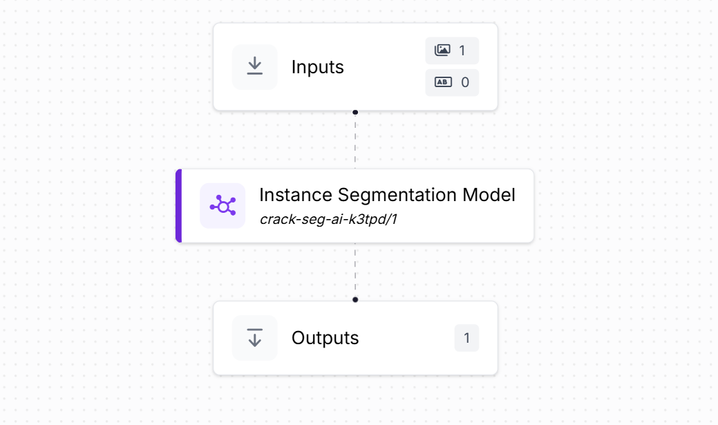
The workflow consists of the following blocks:

• Inputs: Defines the incoming data (an image of a surface that may contain cracks).
• Instance Segmentation Model: Runs the trained crack segmentation model (e.g., crack-seg-ai-k3tpd/1). It outputs the pixel-level outline of each crack as a polygon, along with class predictions.
• Outputs: Produces two types of results:

The output is structured JSON output that gives a detailed model predictions, including:

• Plygon coordinates (x, y) outlining each crack
• Predicted class label (e.g., “crack” or “hairline crack”)
• A unique detection ID for reference
• Parent ID linking the detection back to the source image

This workflow ingests an image, applies the trained crack segmentation model and exports structured polygon data for further analysis, reporting, or integration into structural monitoring systems.

Step #4. Deploy the Roboflow Workflow

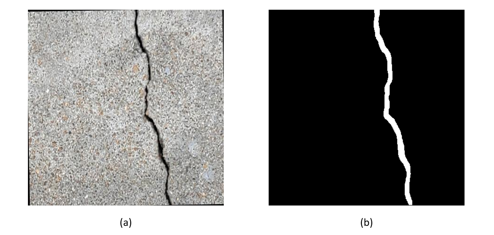
In this step, we deploy the crack segmentation workflow using a simple Python script. The script sends an input image of a surface to the Roboflow Serverless endpoint running the segmentation workflow and receives back polygon predictions outlining the cracks. These predictions are then converted into a binary mask, where the crack regions are highlighted in white against a black background.

Use the code below to run the workflow and generate the crack mask.

import cv2, numpy as np
from inference_sdk import InferenceHTTPClient

# Configure & run your workflow 
API_KEY       = "<ROBOFLOW_API_KEY>"            
WORKSPACE     = "tim-4ijf0"
WORKFLOW_ID   = "crack-segmentation"
IMAGE_INPUT   = "crack.jpg"          

client = InferenceHTTPClient(
    api_url="https://serverless.roboflow.com",
    api_key=API_KEY
)

result = client.run_workflow(
    workspace_name=WORKSPACE,
    workflow_id=WORKFLOW_ID,
    images={"image": IMAGE_INPUT},
    use_cache=False
)

# Extract the "output" dict regardless of schema shape
def extract_output(res):    
    if isinstance(res, dict):
        if "results" in res and res["results"]:
            maybe = res["results"][0]
            if isinstance(maybe, dict) and "output" in maybe:
                return maybe["output"]
        if "output" in res:
            return res["output"] 
    if isinstance(res, list) and len(res) > 0 and isinstance(res[0], dict):
        if "output" in res[0]:
            return res[0]["output"]
    raise KeyError("Could not find 'output' in workflow result. Inspect `result` to adjust key paths.")

out = extract_output(result)

# Pull canvas size and predictions 
W = out["image"]["width"]
H = out["image"]["height"]
preds = out.get("predictions", [])

# Rasterize polygons into a single-channel binary mask (0/255) 
mask = np.zeros((H, W), dtype=np.uint8)

for p in preds:
    pts = p.get("points", [])
    if not pts:
        continue    
    contour = np.array([[pt["x"], pt["y"]] for pt in pts], dtype=np.int32)    
    contour[:, 0] = np.clip(contour[:, 0], 0, W-1) 
    contour[:, 1] = np.clip(contour[:, 1], 0, H-1)  
    contour = contour.reshape((-1, 1, 2))
    cv2.fillPoly(mask, [contour], 255)

# Save outputs 
cv2.imwrite("crack_mask.png", mask)
print("Saved -> crack_mask.png")
print("Mask shape:", mask.shape, "dtype:", mask.dtype, "on-pixels:", int((mask > 0).sum()))

This code demonstrates how to deploy and use a trained crack segmentation workflow to generate a binary mask of cracks from an image. The workflow returns predictions in the form of polygons, where each polygon represents the precise outline of a detected crack. The script extracts these polygon coordinates and rasterizes them onto a blank canvas to create a single-channel binary mask. In this mask, pixels belonging to cracks are filled with white (value 255), while the background remains black (value 0). Finally, the mask is saved as crack_mask.png, and details such as image size and the number of crack pixels are printed. The result is an easy-to-use binary image that isolates cracks from the background, which can be further processed to measure properties such as crack length, width, or area. Running the above code will give you output similar to following:

Now after generating the binary crack mask, the next step is to move from simple detection to measurement. Using the mask as input, the script below analyzes each crack to calculate its length and width.

import cv2
import numpy as np
import matplotlib.pyplot as plt
from skimage.morphology import skeletonize, remove_small_objects, remove_small_holes, medial_axis
from skimage.measure import label, regionprops
import networkx as nx
from math import sqrt, atan2
from pathlib import Path
import pandas as pd
import json

IMAGE_PATH = "crack_mask.png"     # binary/near-binary mask (crack=white, bg=black; auto-fixes inversion)
MIN_REGION_AREA = 64
SAMPLE_EVERY_N_SKELETON_PX = 1
WINDOW_NEIGHBORHOOD = 3
SCALE_MM_PER_PX = None            # e.g., 1.353 to output mm

ORIGINAL_IMAGE_PATH = None        # e.g., "original.jpg"; if None, draw on mask itself

# Visualization (BGR, since we draw in BGR with OpenCV)
SKELETON_THICKNESS = 1
COLOR_SKELETON = (0, 0, 255)      # RED (BGR)
COLOR_WMIN     = (0, 255, 0)      # GREEN (BGR)
COLOR_WMAX     = (255, 0, 0)      # BLUE  (BGR)
WIDTH_HILINE_THICKNESS = 2
DOT_RADIUS = 2
DOT_THICKNESS = -1
FONT = cv2.FONT_HERSHEY_SIMPLEX
LABEL_TEXT_SCALE = 0.35
LABEL_TEXT_THICK = 1

INCLUDE_ENDPOINTS_FOR_WIDTH = False  # keep False for stable widths

# Utilities
def to_rgb(src: np.ndarray) -> np.ndarray:
    if src.ndim == 2:
        return cv2.cvtColor(src, cv2.COLOR_GRAY2RGB)
    if src.ndim == 3 and src.shape[2] == 3:
        return src.copy()
    if src.ndim == 3 and src.shape[2] == 4:
        return cv2.cvtColor(src, cv2.COLOR_RGBA2RGB)
    raise ValueError(f"Unsupported image shape: {src.shape}")

def ensure_binary_mask(img_gray: np.ndarray) -> np.ndarray:
    _, bw = cv2.threshold(img_gray, 0, 255, cv2.THRESH_BINARY + cv2.THRESH_OTSU)
    bw = (bw > 0)
    if bw.mean() > 0.5:  # crack should be minority
        bw = ~bw
    return bw

def clean_mask(mask: np.ndarray) -> np.ndarray:
    mask = remove_small_objects(mask, MIN_REGION_AREA)
    mask = remove_small_holes(mask, area_threshold=MIN_REGION_AREA)
    return mask

def skeleton_graph(skel: np.ndarray):
    ys, xs = np.where(skel)
    coords = list(zip(ys, xs))
    idx_map = -np.ones(skel.shape, dtype=int)
    for i, (y, x) in enumerate(coords):
        idx_map[y, x] = i
    G = nx.Graph()
    for i, (y, x) in enumerate(coords):
        G.add_node(i, y=int(y), x=int(x))
        for dy in (-1, 0, 1):
            for dx in (-1, 0, 1):
                if dy == 0 and dx == 0:
                    continue
                ny, nx_ = y + dy, x + dx
                if 0 <= ny < skel.shape[0] and 0 <= nx_ < skel.shape[1]:
                    j = idx_map[ny, nx_]
                    if j >= 0 and not G.has_edge(i, j):
                        w = sqrt(2.0) if (dx != 0 and dy != 0) else 1.0
                        G.add_edge(i, j, weight=w)
    return G, coords

def skeleton_length_px(G: nx.Graph) -> float:
    return sum(d['weight'] for _, _, d in G.edges(data=True))

def pca_tangent_direction(points):
    pts = np.array(points, dtype=float)
    if pts.shape[0] < 2:
        return 0.0
    pts -= pts.mean(axis=0, keepdims=True)
    C = np.cov(pts.T)
    eigvals, eigvecs = np.linalg.eigh(C)
    principal = eigvecs[:, np.argmax(eigvals)]
    return atan2(principal[0], principal[1])  # (dy, dx) → angle

def local_tangent_angle(skel, y, x, r=3):
    y0, y1 = max(0, y-r), min(skel.shape[0], y+r+1)
    x0, x1 = max(0, x-r), min(skel.shape[1], x+r+1)
    ys, xs = np.where(skel[y0:y1, x0:x1])
    ys = ys + y0
    xs = xs + x0
    if len(ys) < 2:
        return 0.0
    pts = np.stack([ys, xs], axis=1)
    return pca_tangent_direction(pts)

def summarize(arr):
    arr = np.asarray(arr, dtype=float)
    arr = arr[np.isfinite(arr)]
    if arr.size == 0:
        return {}
    return {
        "count": int(arr.size),
        "mean": float(arr.mean()),
        "median": float(np.median(arr)),
        "min": float(arr.min()),
        "max": float(arr.max()),
        "p10": float(np.percentile(arr, 10)),
        "p90": float(np.percentile(arr, 90)),
        "std": float(arr.std(ddof=0)),
    }

# Load & prep
mask_src = cv2.imread(IMAGE_PATH, cv2.IMREAD_GRAYSCALE)
if mask_src is None:
    raise FileNotFoundError(f"Could not read {IMAGE_PATH}")

if ORIGINAL_IMAGE_PATH:
    base_src = cv2.imread(ORIGINAL_IMAGE_PATH, cv2.IMREAD_COLOR)   # BGR
    if base_src is None:
        raise FileNotFoundError(f"Could not read {ORIGINAL_IMAGE_PATH}")
    viz_bgr = base_src.copy()
else:
    base_rgb = to_rgb(mask_src)                                    # RGB
    viz_bgr = cv2.cvtColor(base_rgb, cv2.COLOR_RGB2BGR)            # draw in BGR

raw_mask = ensure_binary_mask(mask_src)
mask = clean_mask(raw_mask)

lab = label(mask)
props = regionprops(lab)
valid_labels = [p.label for p in props if p.area >= MIN_REGION_AREA]
if not valid_labels:
    raise ValueError("No crack components found after cleaning. Try lowering MIN_REGION_AREA.")

# Analyze each component
per_component = []
global_length_px = 0.0
all_widths_px = []
scale = (SCALE_MM_PER_PX if SCALE_MM_PER_PX else 1.0)
unit = "mm" if SCALE_MM_PER_PX else "px"

for idx, comp_id in enumerate(valid_labels, start=1):
    comp_mask = (lab == comp_id)
    if comp_mask.sum() == 0:
        continue

    skel = skeletonize(comp_mask).astype(bool)
    if skel.sum() == 0:
        continue

    # Graph & length
    G, coords = skeleton_graph(skel)
    length_px = skeleton_length_px(G)
    global_length_px += length_px

    # Candidate points for width (degree==2; optionally endpoints)
    node_by_yx = {(G.nodes[n]['y'], G.nodes[n]['x']): n for n in G.nodes()}
    deg = {n: G.degree(n) for n in G.nodes()}
    coords_list = [(int(y), int(x)) for y, x in coords]
    coords_list = [(y, x) for (y, x) in coords_list if deg.get(node_by_yx[(y, x)], 0) == 2] + \
                  ([(y, x) for (y, x) in coords_list if INCLUDE_ENDPOINTS_FOR_WIDTH and deg.get(node_by_yx[(y, x)], 0) == 1])
    if SAMPLE_EVERY_N_SKELETON_PX > 1:
        coords_list = coords_list[::SAMPLE_EVERY_N_SKELETON_PX]

    # Medial-axis width (distance transform)
    skel_ma, dist = medial_axis(comp_mask, return_distance=True)

    widths_px = []
    samples = []  # (y, x, wpx, theta)
    for (y, x) in coords_list:
        wpx = 2.0 * float(dist[y, x])
        if np.isfinite(wpx) and wpx > 0:
            widths_px.append(wpx)
            theta = local_tangent_angle(skel, y, x, r=WINDOW_NEIGHBORHOOD)  # orientation only
            samples.append((y, x, wpx, theta))

    all_widths_px.extend(widths_px)
    wstats_px = summarize(widths_px)
    min_w = wstats_px.get("min", 0.0)
    max_w = wstats_px.get("max", 0.0)

    # Draw ONLY Wmin/Wmax lines, then skeleton in RED ---
    if len(samples) > 0:
        wvals = [s[2] for s in samples]
        i_min = int(np.argmin(wvals))
        i_max = int(np.argmax(wvals))

        for i_sel, col in [(i_min, COLOR_WMIN), (i_max, COLOR_WMAX)]:
            y, x, wpx, theta = samples[i_sel]
            half = 0.5 * wpx
            dy, dx = np.sin(theta + np.pi/2.0), np.cos(theta + np.pi/2.0)
            y1 = int(round(y - dy * half)); x1 = int(round(x - dx * half))
            y2 = int(round(y + dy * half)); x2 = int(round(x + dx * half))
            cv2.line(viz_bgr, (x1, y1), (x2, y2), col, WIDTH_HILINE_THICKNESS)
            cv2.circle(viz_bgr, (int(x), int(y)), DOT_RADIUS, col, DOT_THICKNESS)
            # numeric label only
            val = wpx * scale
            cv2.putText(viz_bgr, f"{val:.2f} {unit}",
                        (int(x) + 6, int(y) - 6),
                        FONT, LABEL_TEXT_SCALE, col, LABEL_TEXT_THICK, cv2.LINE_AA)

    # Skeleton in RED (draw after lines so it's on top if overlapping)
    skel_u8 = (skel.astype(np.uint8) * 255)
    if SKELETON_THICKNESS > 1:
        kernel = cv2.getStructuringElement(cv2.MORPH_ELLIPSE, (SKELETON_THICKNESS, SKELETON_THICKNESS))
        skel_draw = cv2.dilate(skel_u8, kernel)
    else:
        skel_draw = skel_u8
    ys, xs = np.where(skel_draw > 0)
    viz_bgr[ys, xs] = COLOR_SKELETON

    # Component length label near centroid: "C{idx} {value}"
    cy, cx = map(int, np.round(regionprops(comp_mask.astype(np.uint8))[0].centroid))
    cv2.putText(viz_bgr, f"C{idx} {length_px*scale:.1f} {unit}",
                (max(5, cx-60), max(15, cy-10)),
                FONT, LABEL_TEXT_SCALE, COLOR_SKELETON, LABEL_TEXT_THICK, cv2.LINE_AA)

    # Save row
    row = {
        "component_id": idx,
        "pixel_area": int(comp_mask.sum()),
        "length_px": float(length_px),
        "width_min_px": float(min_w),
        "width_max_px": float(max_w),
        "n_width_samples": int(wstats_px.get("count", 0)),
    }
    if SCALE_MM_PER_PX:
        row.update({
            "length_mm": float(length_px * SCALE_MM_PER_PX),
            "width_min_mm": float(min_w * SCALE_MM_PER_PX),
            "width_max_mm": float(max_w * SCALE_MM_PER_PX),
        })
    per_component.append(row)

# Show & save
viz_rgb = cv2.cvtColor(viz_bgr, cv2.COLOR_BGR2RGB)
plt.figure(figsize=(12, 10))
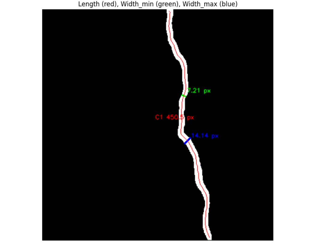
plt.title("Length (red), Width_min (green), Width_max (blue)")
plt.imshow(viz_rgb)
plt.axis('off')
plt.show()

overlay_path = Path("crack_overlay_minmax_skeleton_red_numeric_only.png")
cv2.imwrite(str(overlay_path), cv2.cvtColor(viz_rgb, cv2.COLOR_RGB2BGR))
print(f"Saved overlay: {overlay_path.resolve()}")

df = pd.DataFrame(per_component).sort_values("component_id")
csv_path = Path("crack_component_metrics.csv")
df.to_csv(csv_path, index=False)
print(f"Saved CSV: {csv_path.resolve()}")

report = {
    "pixel_units": {"total_length_px": float(sum(r["length_px"] for r in per_component))},
    "real_units": {
        "scale_mm_per_px": SCALE_MM_PER_PX,
        "total_length_mm": (float(sum(r["length_px"] for r in per_component) * SCALE_MM_PER_PX) if SCALE_MM_PER_PX else None),
    },
    "components": per_component,
    "settings": {
        "min_region_area_px": MIN_REGION_AREA,
        "skeleton_subsample": SAMPLE_EVERY_N_SKELETON_PX,
        "tangent_window_r": WINDOW_NEIGHBORHOOD,
        "include_endpoints_for_width": INCLUDE_ENDPOINTS_FOR_WIDTH,
        "width_method": "medial_axis_distance",
        "viz": "no_mask_fill, skeleton_red, wmin_green, wmax_blue, numeric_labels_only",
    }
}
with open("crack_report.json", "w") as f:
    json.dump(report, f, indent=2)
print("Saved JSON report: crack_report.json")

To measure length, the code applies skeletonization, which reduces each crack to a one-pixel-wide centerline while preserving its overall shape. This skeleton is then treated as a graph, where each pixel is a node connected to its neighbors. By summing the distances along this skeleton graph, the code calculates the total crack length. This is more accurate than simply counting pixels, as it accounts for diagonal connections and curving shapes.

To measure width, the code uses a distance transform. For every skeleton pixel, it calculates how far that pixel is from the nearest crack boundary. Doubling this value gives the local width at that position. By sampling many skeleton points, the code builds a profile of crack widths across the structure. From this, it extracts the minimum width (narrowest section) and maximum width (widest section).

Finally, the code overlays these measurements back onto the image for visual confirmation: the skeleton is drawn in red, the narrowest width line in green, and the widest width line in blue. At the same time, all measurements are saved into CSV and JSON reports, providing both visual and numerical outputs.

When you run the code, you should see output similar to following.

Crack Detection with Vision AI Conclusion

Crack detection using computer vision and deep learning has transformed the way structural health monitoring and quality control are performed across industries. Moving beyond manual inspection and traditional image processing, modern approaches such as classification, object detection, and segmentation offer scalable, accurate, and real-time solutions for identifying cracks in diverse environments.

Practical implementations, from road-mounted cameras to drone-assisted inspections and factory quality control, demonstrate that AI assisted crack detection is not only feasible but highly effective in real-world conditions. With platforms like Roboflow, engineers and researchers can rapidly build, train, and deploy end-to-end systems that adapt to different domains, from tiny hairline fractures in tiles to large pavement and concrete cracks.

Cite this Post

Use the following entry to cite this post in your research:

Timothy M.. (Sep 16, 2025). Crack Detection with Computer Vision. Roboflow Blog: https://blog.roboflow.com/crack-detection/