
OpenCV is the most widely used open-source library for computer vision and image processing in Python, C++, and Java, covering operations from basic color format conversion and resizing to histogram equalization, thresholding, and feature matching with FLANN. This tutorial walks through environment setup, image representation as multi-dimensional arrays, enhancement techniques like blurring and sharpening, and advanced feature-matching using Lowe's ratio test, giving practitioners a grounded foundation for preprocessing images before model training or deployment.
Image processing is a rapidly evolving field that involves manipulating digital images to extract information, enhance visual quality, or prepare images for further analysis. With applications ranging from medical imaging to autonomous vehicles, image processing has become an essential technology in our daily lives.
OpenCV (Open Source Computer Vision Library) is the most widely used open-source library for computer vision and image processing tasks. Created by Intel in 1999, it has evolved into a powerful tool with implementations in multiple languages, including Python, C++, and Java.
In this blog, we'll explore image processing fundamentals using Python with OpenCV, covering everything from basic operations to complex algorithms and real-world applications.
How to Set Up Your Environment for Image Processing with OpenCV
Before we begin, let's set up our Python environment with OpenCV:
# Install OpenCV using pip
# pip install opencv-python numpy matplotlib


# Import the required libraries
import cv2
import numpy as np
import matplotlib.pyplot as plt

# Helper function to display images in the notebook
def display_image(image, title='Image', cmap=None):
    plt.figure(figsize=(10, 8))
    if len(image.shape) == 3:  # Color image
        plt.imshow(cv2.cvtColor(image, cv2.COLOR_BGR2RGB))
    else:  # Grayscale image
        plt.imshow(image, cmap='gray')
    plt.title(title)
    plt.axis('off')
    plt.show()
Understanding Digital Images
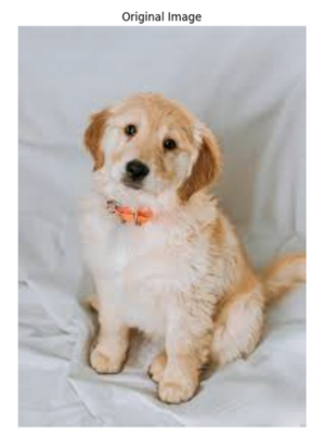
At its core, a digital image is simply a numerical representation of visual information. Understanding how images are represented digitally is crucial for effective image processing.
Image Representation
Images in computers are represented as multi-dimensional arrays:
- Grayscale images: 2D arrays (height × width)
- Color images: 3D arrays (height × width × channels)
Let's examine how to load and inspect images using OpenCV:
# Load an image
image_path = 'sample_image.jpg'
image = cv2.imread(image_path)
# Display basic image information
print(f"Image dimensions (height, width, channels): {image.shape}")
print(f"Image data type: {image.dtype}")
print(f"Image size (bytes): {image.size}")
# Convert to grayscale
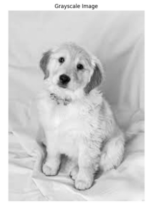
gray_image = cv2.cvtColor(image, cv2.COLOR_BGR2GRAY)
print(f"Grayscale image dimensions: {gray_image.shape}")
# Display the images
display_image(image, "Original Image")
display_image(gray_image, "Grayscale Image")
# Access pixel values
pixel_value = image[100, 100] # Access pixel at (y=100, x=100)
print(f"Pixel value at (100,100): {pixel_value} (BGR format)")
gray_pixel = gray_image[100, 100] # Access pixel in grayscale image
print(f"Grayscale pixel value at (100,100): {gray_pixel}")
1. Image Types and Color Formats in OpenCV
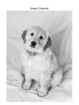
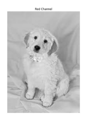
OpenCV loads images in BGR (Blue-Green-Red) format by default, which is different from the more common RGB format. This is an important detail to remember when working with OpenCV.
# Splitting channels
blue, green, red = cv2.split(image)
# Display individual channels
display_image(blue, "Blue Channel", cmap='gray')
display_image(green, "Green Channel", cmap='gray')
display_image(red, "Red Channel", cmap='gray')
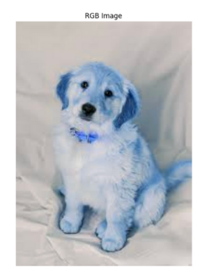
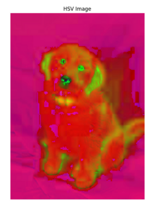
# Converting between color spaces
rgb_image = cv2.cvtColor(image, cv2.COLOR_BGR2RGB)
hsv_image = cv2.cvtColor(image, cv2.COLOR_BGR2HSV)
display_image(rgb_image, "RGB Image")
display_image(hsv_image, "HSV Image")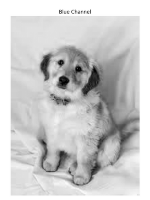
2. Basic Image Operations in OpenCV
Now let's explore fundamental operations that form the building blocks of more complex image processing algorithms.
Image Resizing in OpenCV
Resizing is one of the most common operations in image processing, whether to reduce computational complexity or to standardize input for machine learning models.
# Resize an image
height, width = image.shape[:2]

# Method 1: Specify new dimensions
half_image = cv2.resize(image, (width//2, height//2))

# Method 2: Specify scaling factors
double_image = cv2.resize(image, None, fx=2, fy=2, interpolation=cv2.INTER_CUBIC)

display_image(half_image, "Half Size Image")
display_image(double_image, "Double Size Image")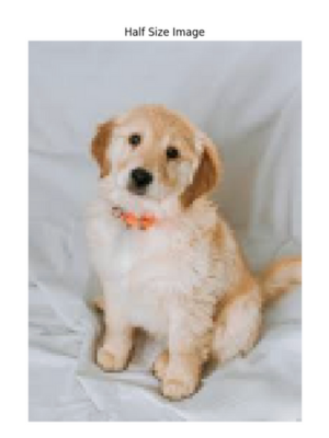
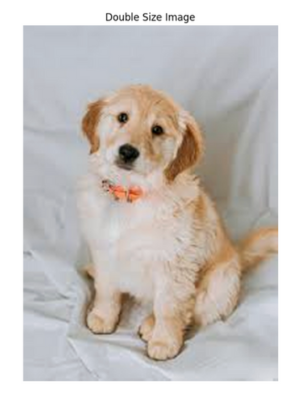
Image Cropping in OpenCV
Extracting regions of interest (ROI) is another fundamental operation:
# Crop an image - format is [y_start:y_end, x_start:x_end]
height, width = image.shape[:2]
center_y, center_x = height//2, width//2
size = 100

# Crop a 200x200 region from the center
cropped_image = image[center_y-size:center_y+size, center_x-size:center_x+size]
display_image(cropped_image, "Cropped Image")
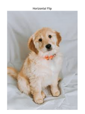
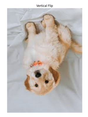
Image Rotation and Flipping
# Rotate an image
height, width = image.shape[:2]
center = (width//2, height//2)
rotation_matrix = cv2.getRotationMatrix2D(center, 45, 1.0)  # 45 degrees
rotated_image = cv2.warpAffine(image, rotation_matrix, (width, height))

# Flip an image
horizontal_flip = cv2.flip(image, 1)  # 1 for horizontal flip
vertical_flip = cv2.flip(image, 0)    # 0 for vertical flip
both_flip = cv2.flip(image, -1)       # -1 for both horizontal and vertical

display_image(rotated_image, "Rotated Image")
display_image(horizontal_flip, "Horizontal Flip")
display_image(vertical_flip, "Vertical Flip")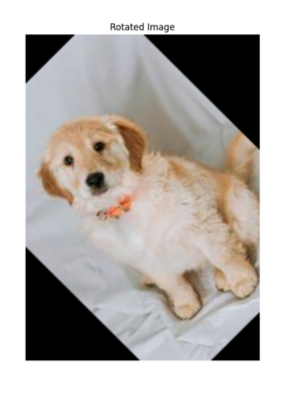
Drawing and Adding Text in OpenCV
OpenCV provides functions to draw shapes and text on images:
# Create a copy to draw on
draw_image = image.copy()

# Draw a rectangle
cv2.rectangle(draw_image, (100, 100), (300, 300), (0, 255, 0), 2)

# Draw a circle
cv2.circle(draw_image, (width//2, height//2), 100, (0, 0, 255), 3)

# Draw a line
cv2.line(draw_image, (0, 0), (width, height), (255, 0, 0), 5)

# Add text
font = cv2.FONT_HERSHEY_SIMPLEX
cv2.putText(draw_image, "OpenCV", (50, 50), font, 1, (255, 255, 255), 2)

display_image(draw_image, "Image with Drawings and Text")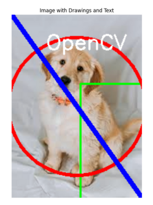
3. Image Enhancement Techniques in OpenCV
Image enhancement improves the visual quality or emphasizes certain features of an image.
Image Smoothing (Blurring)
Blurring helps reduce noise and detail in an image, which is often a preprocessing step for other algorithms.
# Applying different blurring techniques

# 1. Gaussian Blur
gaussian_blur = cv2.GaussianBlur(image, (5, 5), 0)

# 2. Median Blur
median_blur = cv2.medianBlur(image, 5)

# 3. Bilateral Filter (preserves edges while blurring)
bilateral_blur = cv2.bilateralFilter(image, 9, 75, 75)

display_image(gaussian_blur, "Gaussian Blur")
display_image(median_blur, "Median Blur")
display_image(bilateral_blur, "Bilateral Filter")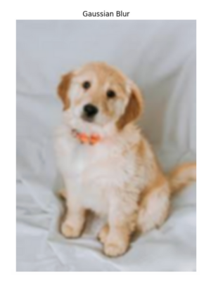
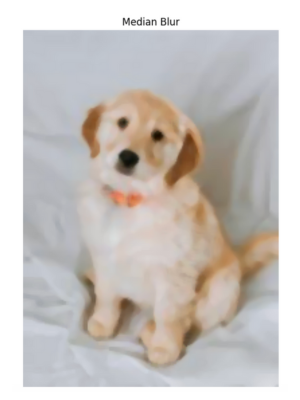

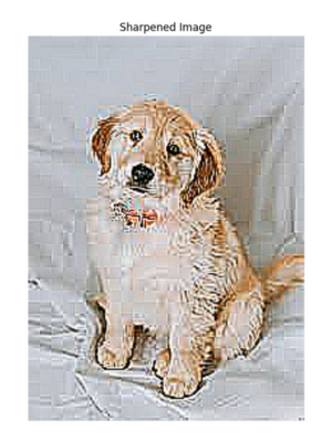
Image Sharpening
Sharpening enhances edges and details in an image making it appear clearer.
# Sharpening using kernel
kernel = np.array([[-1, -1, -1],
                   [-1,  9, -1],
                   [-1, -1, -1]])
sharpened = cv2.filter2D(image, -1, kernel)
display_image(sharpened, "Sharpened Image")
Histogram Equalization
Ideal for low contrast or poorly lit images, this technique improves contrast by redistributing intensity values more evenly across the available range:
# Histogram equalization works best on grayscale images
gray_image = cv2.cvtColor(image, cv2.COLOR_BGR2GRAY)
equalized = cv2.equalizeHist(gray_image)
# Display histograms
fig, axes = plt.subplots(2, 2, figsize=(15, 10))
axes[0, 0].imshow(gray_image, cmap='gray')
axes[0, 0].set_title('Original Grayscale Image')
axes[0, 0].axis('off')
axes[0, 1].imshow(equalized, cmap='gray')
axes[0, 1].set_title('Equalized Image')
axes[0, 1].axis('off')
axes[1, 0].hist(gray_image.ravel(), 256, [0, 256])
axes[1, 0].set_title('Histogram of Original Image')
axes[1, 1].hist(equalized.ravel(), 256, [0, 256])
axes[1, 1].set_title('Histogram of Equalized Image')
plt.tight_layout()
plt.show()
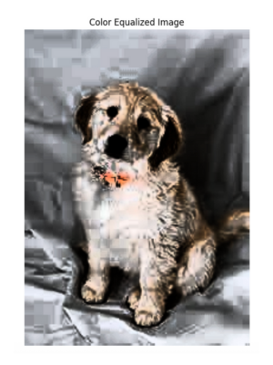
# For color images, apply equalization to the V channel in HSV space
hsv_image = cv2.cvtColor(image, cv2.COLOR_BGR2HSV)
hsv_image[:,:,2] = cv2.equalizeHist(hsv_image[:,:,2])
equalized_color = cv2.cvtColor(hsv_image, cv2.COLOR_HSV2BGR)
display_image(equalized_color, "Color Equalized Image")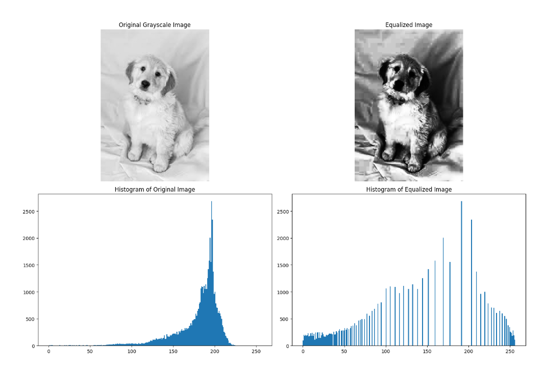
4. Thresholding and Binary Images
Thresholding converts a grayscale image into a binary image, which is crucial for many computer vision tasks, for example in document scanning.
Basic Thresholding
# Convert to grayscale
gray_image = cv2.cvtColor(image, cv2.COLOR_BGR2GRAY)

# Apply simple thresholding
_, binary_image = cv2.threshold(gray_image, 127, 255, cv2.THRESH_BINARY)
_, binary_inv = cv2.threshold(gray_image, 127, 255, cv2.THRESH_BINARY_INV)
_, trunc = cv2.threshold(gray_image, 127, 255, cv2.THRESH_TRUNC)
_, to_zero = cv2.threshold(gray_image, 127, 255, cv2.THRESH_TOZERO)

# Display results
fig, axes = plt.subplots(2, 3, figsize=(15, 10))
axes = axes.ravel()

axes[0].imshow(gray_image, cmap='gray')
axes[0].set_title('Original')
axes[0].axis('off')

axes[1].imshow(binary_image, cmap='gray')
axes[1].set_title('Binary')
axes[1].axis('off')

axes[2].imshow(binary_inv, cmap='gray')
axes[2].set_title('Binary Inverted')
axes[2].axis('off')

axes[3].imshow(trunc, cmap='gray')
axes[3].set_title('Truncated')
axes[3].axis('off')

axes[4].imshow(to_zero, cmap='gray')
axes[4].set_title('To Zero')
axes[4].axis('off')

plt.tight_layout()
plt.show()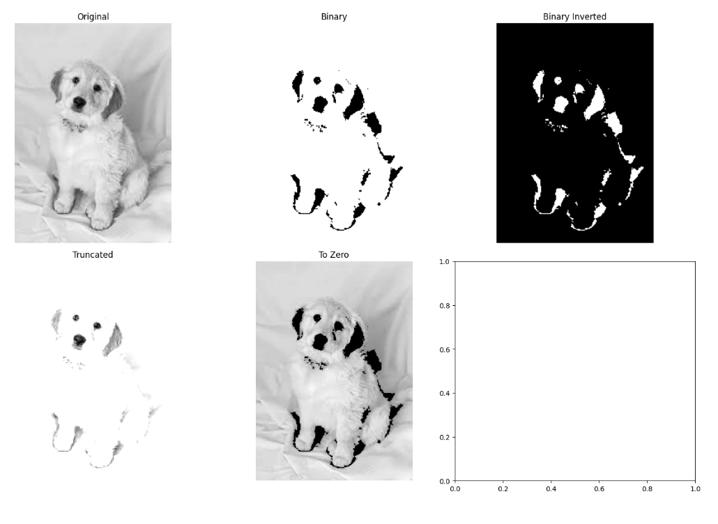
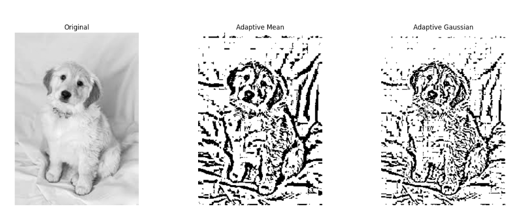
Adaptive Thresholding
When an image has uneven lighting, shadows, or gradients, adaptive thresholding can be very useful. Adaptive thresholding calculates the threshold for smaller regions of the image, which gives better results for images with varying illumination:
# Apply adaptive thresholding
adaptive_mean = cv2.adaptiveThreshold(gray_image, 255,
                                      cv2.ADAPTIVE_THRESH_MEAN_C,
                                      cv2.THRESH_BINARY, 11, 2)

adaptive_gaussian = cv2.adaptiveThreshold(gray_image, 255,
                                          cv2.ADAPTIVE_THRESH_GAUSSIAN_C,
                                          cv2.THRESH_BINARY, 11, 2)

# Display results
fig, axes = plt.subplots(1, 3, figsize=(15, 5))

axes[0].imshow(gray_image, cmap='gray')
axes[0].set_title('Original')
axes[0].axis('off')

axes[1].imshow(adaptive_mean, cmap='gray')
axes[1].set_title('Adaptive Mean')
axes[1].axis('off')

axes[2].imshow(adaptive_gaussian, cmap='gray')
axes[2].set_title('Adaptive Gaussian')
axes[2].axis('off')

plt.tight_layout()
plt.show()
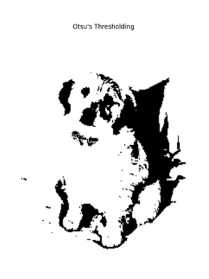
Otsu's Thresholding
Otsu's method automatically calculates an optimal threshold value. This is particularly useful for images with bimodal histograms and when you don't know the right threshold value.
# Apply Otsu's thresholding
_, otsu = cv2.threshold(gray_image, 0, 255, cv2.THRESH_BINARY + cv2.THRESH_OTSU)
display_image(otsu, "Otsu's Thresholding")
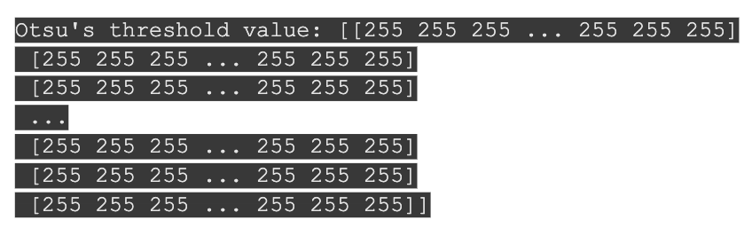
# Print the threshold value calculated by Otsu's method
_, otsu_thresh_value = cv2.threshold(gray_image, 0, 255, cv2.THRESH_BINARY + cv2.THRESH_OTSU)
print(f"Otsu's threshold value: {otsu_thresh_value}")
5. Edge Detection and Contour Detection
Edge detection identifies boundaries within an image, while contour detection finds the outlines of objects. Edge detection is useful for identifying sudden changes in pixel intensity, which typically corresponds to object boundaries, texture changes, shape outlines, depth changes, and shadows or lighting transitions. Contour detection can help identify the shape, size, and position of objects in an image.
Edge Detection
# Apply various edge detection methods

# Sobel edge detection
sobelx = cv2.Sobel(gray_image, cv2.CV_64F, 1, 0, ksize=3)  # x direction
sobely = cv2.Sobel(gray_image, cv2.CV_64F, 0, 1, ksize=3)  # y direction
sobelx = cv2.convertScaleAbs(sobelx)
sobely = cv2.convertScaleAbs(sobely)
sobel_combined = cv2.addWeighted(sobelx, 0.5, sobely, 0.5, 0)

# Laplacian edge detection
laplacian = cv2.Laplacian(gray_image, cv2.CV_64F)
laplacian = cv2.convertScaleAbs(laplacian)

# Canny edge detection
canny = cv2.Canny(gray_image, 100, 200)

# Display results
fig, axes = plt.subplots(2, 3, figsize=(15, 10))
axes = axes.flatten()

axes[0].imshow(gray_image, cmap='gray')
axes[0].set_title('Original')
axes[0].axis('off')

axes[1].imshow(sobelx, cmap='gray')
axes[1].set_title('Sobel X')
axes[1].axis('off')

axes[2].imshow(sobely, cmap='gray')
axes[2].set_title('Sobel Y')
axes[2].axis('off')

axes[3].imshow(sobel_combined, cmap='gray')
axes[3].set_title('Sobel Combined')
axes[3].axis('off')

axes[4].imshow(laplacian, cmap='gray')
axes[4].set_title('Laplacian')
axes[4].axis('off')

axes[5].imshow(canny, cmap='gray')
axes[5].set_title('Canny')
axes[5].axis('off')

plt.tight_layout()
plt.show()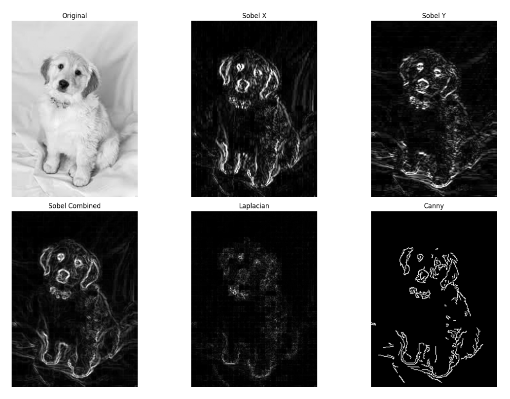
Contour Detection
Contours are useful for shape analysis, object detection, and recognition:
# Find contours in an image
# First create a binary image
_, binary = cv2.threshold(gray_image, 127, 255, cv2.THRESH_BINARY)
contours, hierarchy = cv2.findContours(binary, cv2.RETR_TREE, cv2.CHAIN_APPROX_SIMPLE)
# Draw all contours
contour_image = image.copy()
cv2.drawContours(contour_image, contours, -1, (0, 255, 0), 2)
display_image(contour_image, "All Contours")
# Draw only the largest contour
largest_contour = max(contours, key=cv2.contourArea)
largest_contour_image = image.copy()
cv2.drawContours(largest_contour_image, [largest_contour], 0, (0, 0, 255), 3)
display_image(largest_contour_image, "Largest Contour")
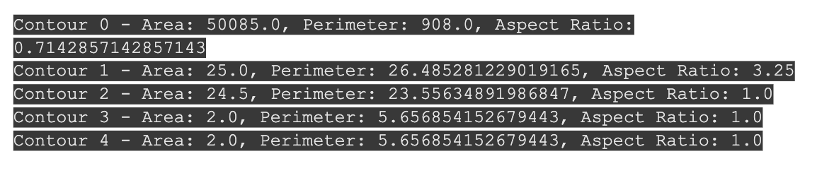
# Getting contour properties
for i, contour in enumerate(contours[:5]): # Look at the first 5 contours only
area = cv2.contourArea(contour)
perimeter = cv2.arcLength(contour, True)
# Find bounding shapes
x, y, w, h = cv2.boundingRect(contour)
aspect_ratio = float(w) / h
# Print contour information
print(f"Contour {i} - Area: {area}, Perimeter: {perimeter}, Aspect Ratio: {aspect_ratio}")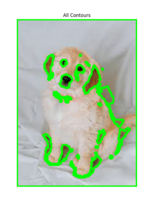

6. Morphological Operations
Morphological operations process images based on their shapes. They're particularly useful for processing binary and grayscale images.
Basic Morphological Operations
# Create a simple binary image
_, binary = cv2.threshold(gray_image, 127, 255, cv2.THRESH_BINARY_INV)

# Define kernel (structuring element)
kernel = np.ones((5,5), np.uint8)

# Apply morphological operations
erosion = cv2.erode(binary, kernel, iterations=1)
dilation = cv2.dilate(binary, kernel, iterations=1)
opening = cv2.morphologyEx(binary, cv2.MORPH_OPEN, kernel)  # Erosion followed by dilation
closing = cv2.morphologyEx(binary, cv2.MORPH_CLOSE, kernel)  # Dilation followed by erosion
gradient = cv2.morphologyEx(binary, cv2.MORPH_GRADIENT, kernel)  # Difference between dilation and erosion

# Display results
fig, axes = plt.subplots(2, 3, figsize=(15, 10))
axes = axes.flatten()

axes[0].imshow(binary, cmap='gray')
axes[0].set_title('Binary Image')
axes[0].axis('off')

axes[1].imshow(erosion, cmap='gray')
axes[1].set_title('Erosion')
axes[1].axis('off')

axes[2].imshow(dilation, cmap='gray')
axes[2].set_title('Dilation')
axes[2].axis('off')

axes[3].imshow(opening, cmap='gray')
axes[3].set_title('Opening')
axes[3].axis('off')

axes[4].imshow(closing, cmap='gray')
axes[4].set_title('Closing')
axes[4].axis('off')

axes[5].imshow(gradient, cmap='gray')
axes[5].set_title('Morphological Gradient')
axes[5].axis('off')

plt.tight_layout()
plt.show()
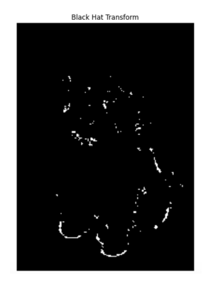
Advanced Morphological Operations
Advanced morphological operations are helpful when you need fine control over shapes and structures in a binary image.
# Top Hat and Black Hat transforms
top_hat = cv2.morphologyEx(binary, cv2.MORPH_TOPHAT, kernel) # Difference between input and opening
black_hat = cv2.morphologyEx(binary, cv2.MORPH_BLACKHAT, kernel) # Difference between closing and input
display_image(top_hat, "Top Hat Transform")
display_image(black_hat, "Black Hat Transform")
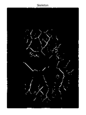
# Skeleton extraction
def skeletonize(img):
size = np.size(img)
skeleton = np.zeros(img.shape, np.uint8)
ret, img = cv2.threshold(img, 127, 255, 0)
element = cv2.getStructuringElement(cv2.MORPH_CROSS, (3,3))
done = False
while not done:
eroded = cv2.erode(img, element)
temp = cv2.dilate(eroded, element)
temp = cv2.subtract(img, temp)
skeleton = cv2.bitwise_or(skeleton, temp)
img = eroded.copy()
zeros = size - cv2.countNonZero(img)
if zeros == size:
done = True
return skeleton
skeleton = skeletonize(binary)
display_image(skeleton, "Skeleton")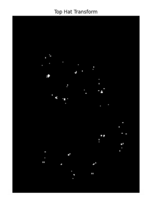
7. Color Spaces and Object Detection
Color spaces are different ways to represent colors in images. OpenCV supports various color spaces that are useful for different applications.
Color Space Conversions
# Convert between color spaces
bgr_image = image.copy()
rgb_image = cv2.cvtColor(bgr_image, cv2.COLOR_BGR2RGB)
hsv_image = cv2.cvtColor(bgr_image, cv2.COLOR_BGR2HSV)
lab_image = cv2.cvtColor(bgr_image, cv2.COLOR_BGR2LAB)
gray_image = cv2.cvtColor(bgr_image, cv2.COLOR_BGR2GRAY)

# Display each color space
fig, axes = plt.subplots(2, 2, figsize=(15, 10))
axes = axes.flatten()

axes[0].imshow(cv2.cvtColor(bgr_image, cv2.COLOR_BGR2RGB))
axes[0].set_title('RGB Image')
axes[0].axis('off')

# For HSV and LAB, we need to display individual channels
h, s, v = cv2.split(hsv_image)
hsv_display = np.concatenate([h, s, v], axis=1)
axes[1].imshow(hsv_display, cmap='gray')
axes[1].set_title('HSV Channels (H, S, V)')
axes[1].axis('off')

l, a, b = cv2.split(lab_image)
lab_display = np.concatenate([l, a, b], axis=1)
axes[2].imshow(lab_display, cmap='gray')
axes[2].set_title('LAB Channels (L, A, B)')
axes[2].axis('off')

axes[3].imshow(gray_image, cmap='gray')
axes[3].set_title('Grayscale Image')
axes[3].axis('off')

plt.tight_layout()
plt.show()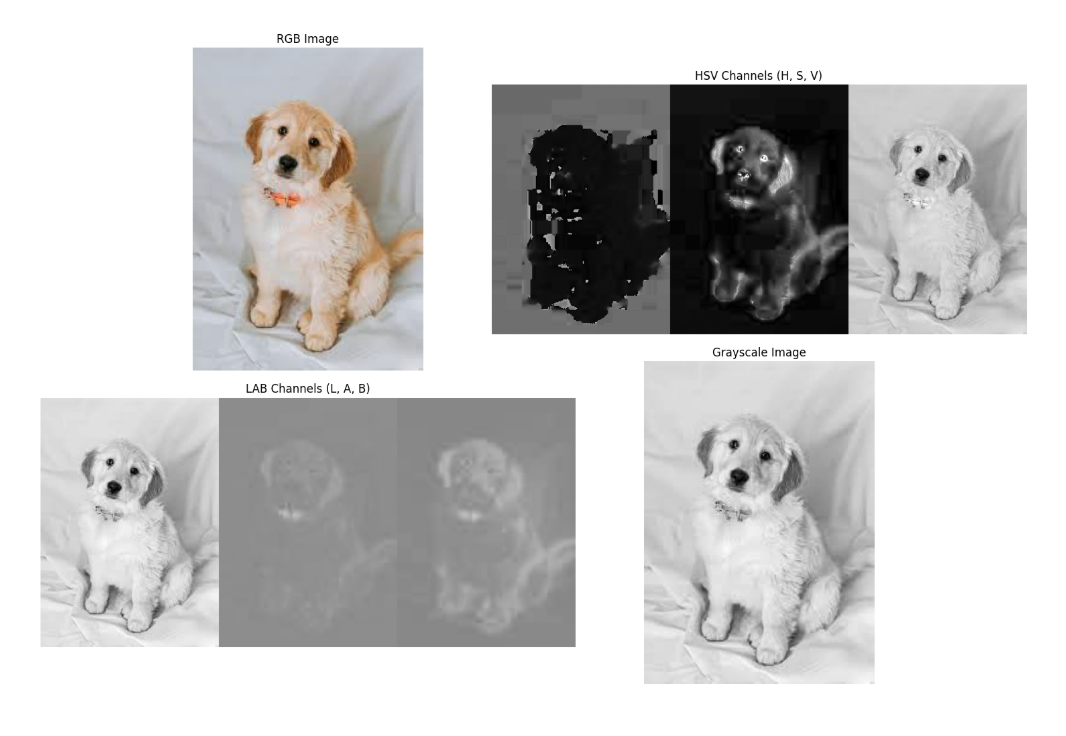
Color-Based Object Detection in OpenCV
One of the simplest ways to detect objects is by their color. HSV color space is particularly useful for this task:
# Define range of a specific color in HSV
# For example, detecting red objects
hsv_image = cv2.cvtColor(image, cv2.COLOR_BGR2HSV)
# Define range for red color (hue is circular, so red is at both low and high ends)
lower_red1 = np.array([0, 100, 100])
upper_red1 = np.array([10, 255, 255])
lower_red2 = np.array([160, 100, 100])
upper_red2 = np.array([180, 255, 255])
# Create masks for red regions
mask1 = cv2.inRange(hsv_image, lower_red1, upper_red1)
mask2 = cv2.inRange(hsv_image, lower_red2, upper_red2)
red_mask = mask1 + mask2
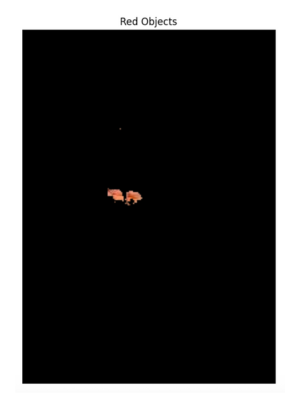
# Apply the mask to extract red objects
red_objects = cv2.bitwise_and(image, image, mask=red_mask)
# Display the results
display_image(red_mask, "Red Mask")
display_image(red_objects, "Red Objects")
# Find contours of detected objects
contours, _ = cv2.findContours(red_mask, cv2.RETR_EXTERNAL, cv2.CHAIN_APPROX_SIMPLE)
# Draw bounding boxes around detected objects
result_image = image.copy()
for contour in contours:
# Filter out small contours
if cv2.contourArea(contour) > 500: # Minimum area threshold
x, y, w, h = cv2.boundingRect(contour)
cv2.rectangle(result_image, (x, y), (x+w, y+h), (0, 255, 0), 2)
display_image(result_image, "Detected Red Objects")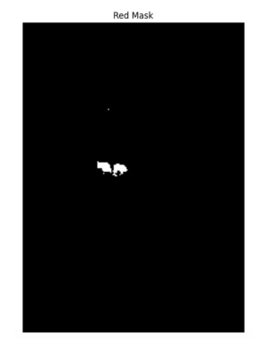

8. Feature Detection and Matching
Feature detection identifies interesting points in an image that can be used for tasks like object recognition, panorama stitching, and 3D reconstruction.
Corner Detection
# Harris Corner Detection
gray_image = cv2.cvtColor(image, cv2.COLOR_BGR2GRAY)
gray_float = np.float32(gray_image)
corners = cv2.cornerHarris(gray_float, blockSize=2, ksize=3, k=0.04)
# Dilate to mark the corners
corners_dilated = cv2.dilate(corners, None)
# Threshold for optimal value (corners > 0.01*corners.max())
threshold = 0.01 * corners.max()
corner_image = image.copy()
corner_image[corners_dilated > threshold] = [0, 0, 255] # Mark corners in red
display_image(corner_image, "Harris Corners")
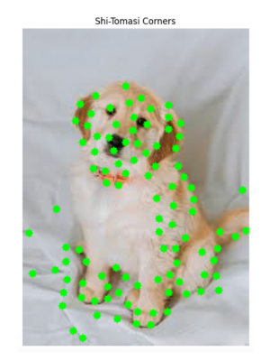
# Shi-Tomasi Corner Detection
corners = cv2.goodFeaturesToTrack(gray_image, maxCorners=100, qualityLevel=0.01, minDistance=10)
corners = np.int0(corners)
shi_tomasi_image = image.copy()
for corner in corners:
x, y = corner.ravel()
cv2.circle(shi_tomasi_image, (x, y), 3, [0, 255, 0], -1)
display_image(shi_tomasi_image, "Shi-Tomasi Corners")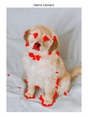
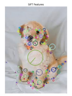
SIFT Feature Detection
Scale-Invariant Feature Transform (SIFT) is a powerful algorithm for detecting and describing local features in images. It can be particularly helpful when you want to detect and describe distinct, repeatable features in an image.
# Initialize SIFT detector
sift = cv2.SIFT_create()
# Detect keypoints and compute descriptors
keypoints, descriptors = sift.detectAndCompute(gray_image, None)
# Draw keypoints
sift_image = cv2.drawKeypoints(image, keypoints, None, flags=cv2.DRAW_MATCHES_FLAGS_DRAW_RICH_KEYPOINTS)
display_image(sift_image, "SIFT Features")
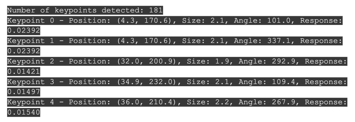
# Print information about detected keypoints
print(f"Number of keypoints detected: {len(keypoints)}")
for i, keypoint in enumerate(keypoints[:5]): # Show first 5 keypoints
print(f"Keypoint {i} - Position: ({keypoint.pt[0]:.1f}, {keypoint.pt[1]:.1f}), " +
f"Size: {keypoint.size:.1f}, Angle: {keypoint.angle:.1f}, Response: {keypoint.response:.5f}")
Feature Matching in OpenCV
Feature matching is useful when you need to connect or compare similar features across multiple images, often to find relationships, transformations, or verify that the same object or scene is present in both. Feature matching finds correspondences between keypoints in different images:
# Load two images
image1 = cv2.imread('image1.jpg', cv2.IMREAD_GRAYSCALE)
image2 = cv2.imread('image2.jpg', cv2.IMREAD_GRAYSCALE)

# Detect SIFT features
sift = cv2.SIFT_create()
keypoints1, descriptors1 = sift.detectAndCompute(image1, None)
keypoints2, descriptors2 = sift.detectAndCompute(image2, None)

# FLANN matching
FLANN_INDEX_KDTREE = 1
index_params = dict(algorithm=FLANN_INDEX_KDTREE, trees=5)
search_params = dict(checks=50)
flann = cv2.FlannBasedMatcher(index_params, search_params)
matches = flann.knnMatch(descriptors1, descriptors2, k=2)

# Apply ratio test
good_matches = []
for m, n in matches:
    if m.distance < 0.7 * n.distance:  # Lowe's ratio test
        good_matches.append(m)

# Draw matches
match_image = cv2.drawMatches(image1, keypoints1, image2, keypoints2, good_matches, None)
display_image(match_image, "Feature Matching")
Image Processing with OpenCV
OpenCV's extensive documentation and community resources make it an ideal platform for continuous learning and development in the exciting field of computer vision.
Remember that image processing is both a science and an art—while algorithms provide the technical foundation, finding the right approach for a specific problem often requires experimentation, creativity, and domain knowledge. Happy learning.
Integrate advanced preprocessing capabilities like resizing, augmentation, and transformation, ensuring your images are in perfect shape for model training and deployment, using Roboflow Annotate. Get started free today.
You might also enjoy learning how to save an image with cv2.imwrite and show images with cv2 imshow.
Cite this Post
Use the following entry to cite this post in your research:
Contributing Writer. (Apr 24, 2025). Image Processing with OpenCV. Roboflow Blog: https://blog.roboflow.com/image-processing-with-opencv/