How to Train a YOLO26 Oriented Bounding Box (OBB) Model

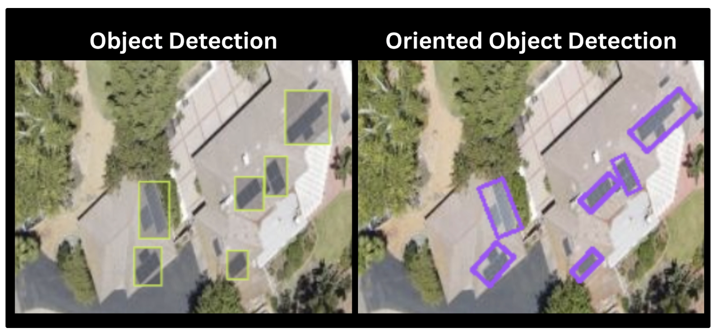
Oriented Bounding Box (OBB) detection is a type of object detection in which a model predicts both the bounding box coordinates and a rotation angle, allowing the bounding box to align with the object’s actual orientation in the image.In standard object detection, models produce axis-aligned bounding boxes that remain horizontal regardless of how an object is positioned. As a result, tilted or rotated objects often lead to loose boxes with excess background, reducing localization accuracy.

OBB models such as YOLO26-OBB address this limitation by predicting rotated bounding boxes that follow the object’s direction. This enables tighter and more precise localization, particularly in use cases like aerial imagery.Instead of only identifying where an object is located, OBB detection also captures how it is oriented, providing a more precise representation of objects in real-world conditions.

Training a YOLO26 Oriented Bounding Box (OBB) Model

In this guide, we will learn how to train a YOLO26 Oriented Bounding Box (OBB) model using a custom aerial image dataset to detect solar panels.

Such a model can be valuable for aerial surveying applications, helping organizations better analyze and understand solar panel adoption across large geographic regions.

Why use Oriented Bounding Box (OBB) Detection?

Better Fit for Rotated Objects: OBB models align bounding boxes with the object’s orientation, reducing unnecessary background space around tilted objects.

• Improved Detection Accuracy: It provides tighter localization compared to axis-aligned boxes, especially for rotated objects.
• Useful for Aerial and Satellite Images: It works well for scenes where objects like buildings, ships, and vehicles appear at different angles.
• More Reliable in Industrial Inspection: It helps detect and analyze parts that are rotated or inconsistently positioned in manufacturing settings.
• Cleaner Object Separation: It reduces overlap confusion when objects are close together or partially rotated.
• Better Representation of Real-World Scenes: It captures both position and orientation, giving a more realistic view of objects in real environments.
• More Efficient than Segmentation for Orientation Tasks: OBB models directly predict object angles using a lightweight representation, making them faster and simpler than using segmentation masks followed by post-processing for rotation estimation.

What is YOLO26?

YOLO26 is a multi-task model family designed to support a wide range of computer vision tasks, including object detection, oriented object detection, instance segmentation, image classification, and pose estimation.

The model lineup includes multiple sizes, Nano (N), Small (S), Medium (M), Large (L), and Extra Large (X), allowing users to choose between faster performance or higher accuracy depending on deployment needs.

Compared to earlier YOLO generations, YOLO26 is optimized for edge deployment with faster CPU inference, a more compact architecture, and improved compatibility across diverse hardware environments.

By default, YOLO models detect COCO classes, but they can be trained on labeled datasets to recognize objects outside of COCO classes, such as solar panels.During training, the model learns by processing annotated images, comparing its predictions with ground truth labels, calculating errors, and iteratively updating its internal weights to improve accuracy over time.

In this guide, we use the YOLO26 Nano OBB model (yolo26n-obb.pt) because it offers an efficient balance between training speed and detection performance, making it well suited for experimentation in Google Colab.

You can learn more about YOLO26 in this blog: YOLO26 blog, and you can try it in the Roboflow Playground: Roboflow Playground.

Training a YOLO26 Oriented Bounding Box (OBB) Model for Solar Panel Detection in Aerial Imagery

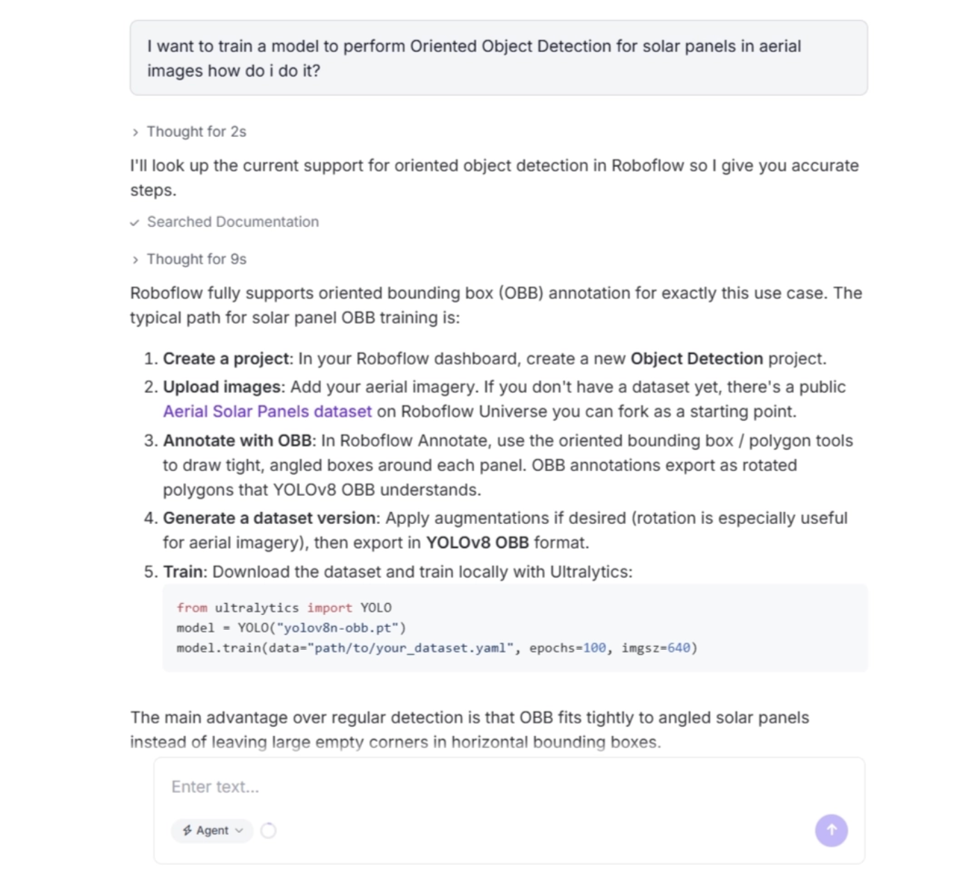
The steps below show how to create and annotate an aerial dataset, then train a model on it to detect both solar panels and their orientation.You can also try Roboflow Agent, available in your workspace. It is a conversational chatbot built on top of Roboflow’s tools, such as Workflows, where you can describe computer vision models or workflows in plain English, and it will handle the process of building them for you.

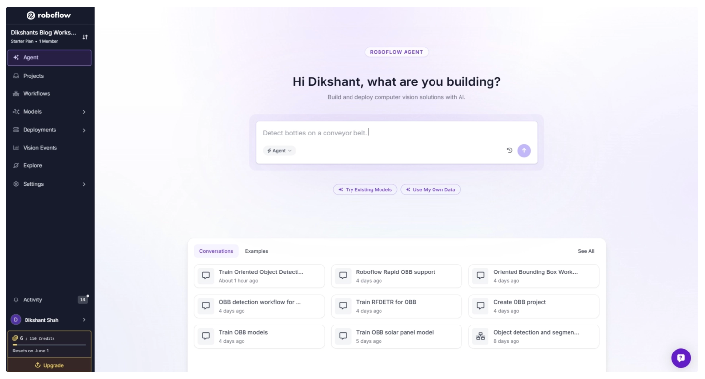
In our case, it can be used as an AI agent to suggest improvements, help troubleshoot issues, and recommend steps for the YOLO26-OBB training process, as shown below.

Step 1: Create a Roboflow Project

To train a model we need a dataset of labeled images with oriented bounding boxes so that our model can learn exactly where objects of interest are in an image. To begin compiling a dataset of images and start labeling them, we first need to create a Roboflow Project.

To create a project, first create a free Roboflow account and log in. Then, in your workspace, go to the left-sidebar menu, choose “Projects”, and then “+ New Project”.

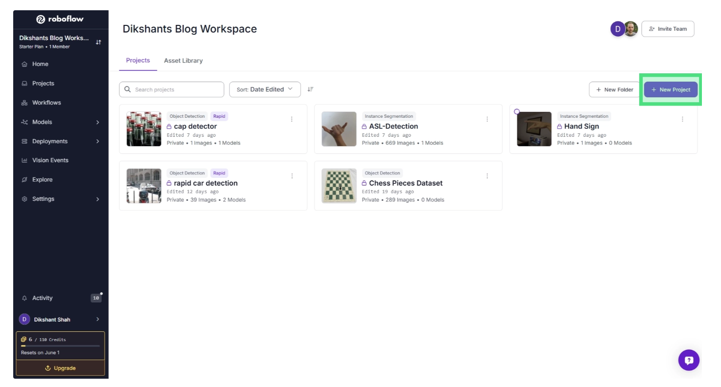
This will open a menu where you can name the project and select the type of project you will be working on. In our case, since this is an OBB project, select “Object Detection” as the project type.

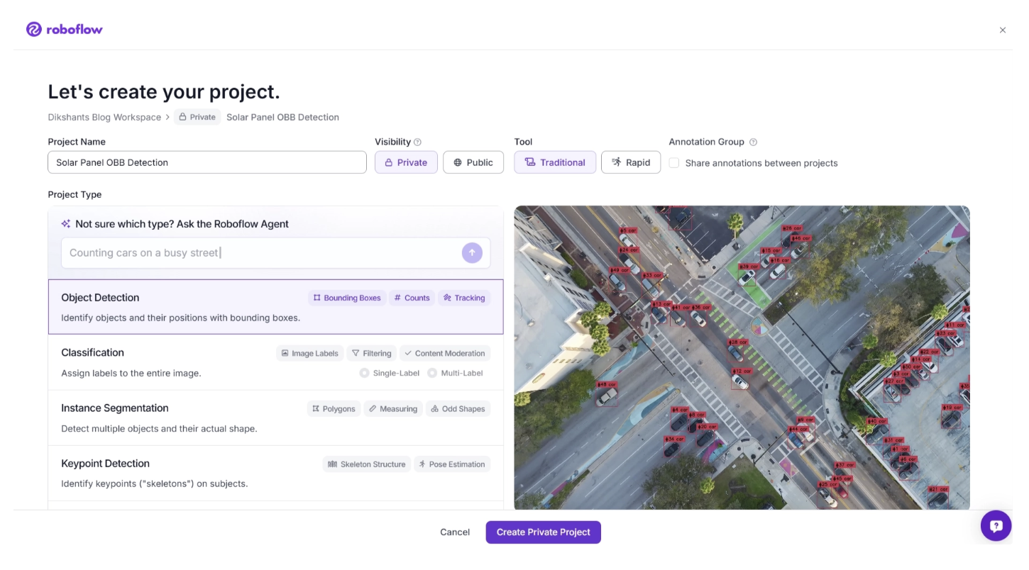
Once you select the project type and click “Create Project,” your project will be created, and you can upload images to annotate and add them to your training dataset.

Step 2: Build a Labeled Dataset

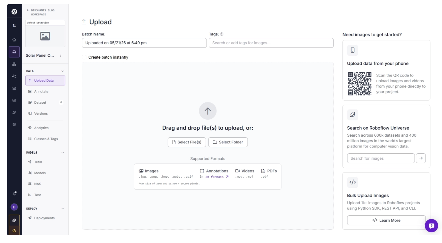
You can drag and drop multiple images to the project as shown below in order to label it as a part of dataset, as shown below.

Once the images are uploaded, Roboflow Annotate offers you various ways to annotate them for training models, such as:

• Label Myself - Manually annotate the images yourself.
• Label With My Team - Collaborate with team members to annotate images together.
• Hire Outsourced Labelers - Use professional external annotators to label the dataset.
• Auto-Label Entire Batch - Automatically generate annotations using AI models such as SAM 3Roboflow Annotate is a web-based tool for labeling images and videos by drawing and managing annotations to build datasets for training computer vision models.

For this guide, we chose the “Label Myself” option, as shown below, where we create oriented bounding boxes around the objects of interest (solar panels) in the image using the Polygon Tool available in the floating menu on the right.

Inside Roboflow Annotate, you can also use the Smart Select tool, an AI-assisted feature powered by the Segment Anything Model 3 (SAM 3) to automatically generate bounding boxes.

This removes the need to manually annotate objects of interest in the image, significantly speeding up the annotation process, as demonstrated below.

Step 3: Download a Dataset from Roboflow Universe

To train a model, we need a large number of annotated images. You can either collect and label your own dataset using Roboflow Annotate as shown in the previous step, or use an existing annotated dataset from Roboflow Universe.

Roboflow Universe is an online, community-driven platform for sharing and discovering computer vision datasets and pre-trained models. It acts as a central hub where developers, researchers, and companies can access open-source image data and annotated datasets for tasks such as object detection, image classification, oriented object detection, segmentation, and more.Roboflow Universe hosts over 1 million+ public computer vision datasets shared by the community, with new datasets added regularly.

In this guide, we will use the Aerial Solar Panels dataset (as shown below), which contains aerial images of solar panels collected via a DJI Mavic Air 2 flying over Rancho Santa Fe, California. This dataset already includes oriented bounding box annotations, so no additional labeling is required.

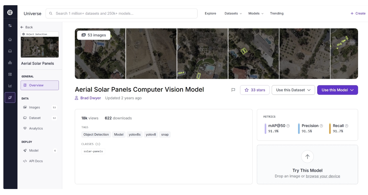
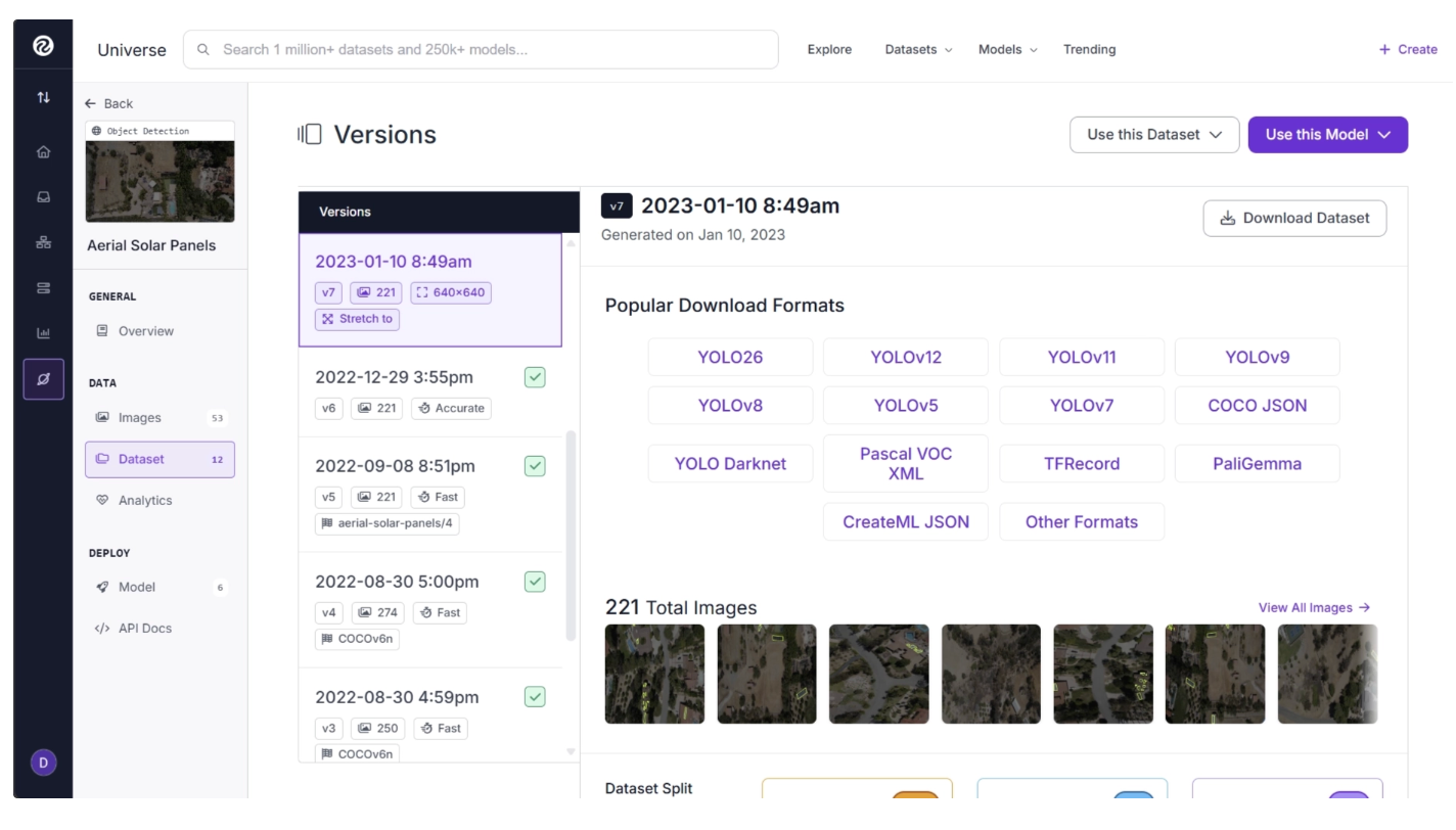
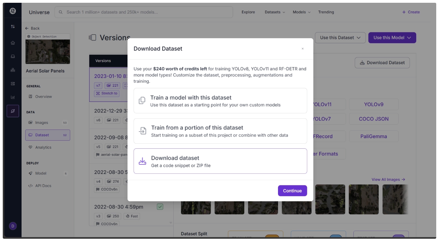
You can download this dataset by clicking “Dataset” under the Data section in the left sidebar menu on the dataset page. From there, you can find different versions of the dataset, select the one you want, and click “Download Dataset”.

This should open up a menu with different options for downloading the dataset. For now, select “Download Dataset”.

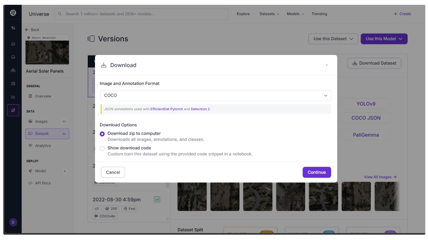
Choose the “Download zip to computer” option.

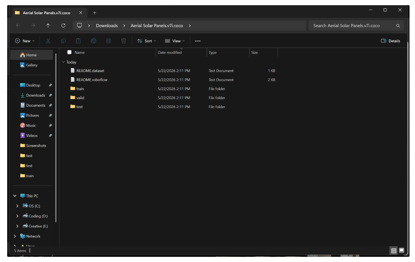
The dataset will be downloaded as a ZIP file. Extract it, and inside you will find the images already split into train, validation, and test folders.

Next, drag and drop the entire extracted “Aerial Solar Panels” folder (including the train, valid, and test directories) into your Roboflow project.

After uploading, save the dataset. Roboflow will automatically recognize the folder structure and assign images to the correct splits (train, valid, and test).

Once saved, it immediately redirects you to the Versions tab, where you can generate a new dataset version for training your model.

You can also view the uploaded dataset by clicking Dataset in the left sidebar, as shown below.

The other direct ways you can use this dataset are by forking or cloning it. Forking creates an editable copy that you can modify and train, while cloning lets you copy the images into your own project.

Step 4: Create a Dataset Version

Once you have labeled your data, you can create a dataset version. A dataset version is a snapshot of your dataset at a specific point in time, allowing you to preserve and manage changes as your dataset evolves.

Dataset versions help you:

• Track changes as you improve or expand your dataset
• Reproduce training results exactly at a later stage
• Compare model performance across different dataset iterations
• Roll back to a previous state if something goes wrong

While creating a dataset version, you can adjust the train, test, and validation splits. You can also apply preprocessing and augmentation steps.

Preprocessing includes operations such as resizing images, converting to grayscale, or applying dynamic crops, while augmentation includes transformations like brightness adjustments, rotation, blur and other variations.

To learn more about preprocessing and augmentation, refer to our image preprocessing and augmentation guides.

To create a dataset version, click Versions in the left sidebar of your Roboflow project, as shown below.

For this guide, we applied a preprocessing step of Auto-Orient and resized all images by stretching them to a 640×640 resolution.After configuring your dataset version, click Continue as shown in the video. Your dataset version will then be generated.

Step 5: Export the Dataset for Training

As of 05/22/2026, Roboflow Train does not support training oriented bounding box (OBB) detection models.

It currently supports training object detection, instance segmentation, classification, semantic segmentation, and keypoint detection models.

If you click Train Model, it will train a standard object detection model that predicts axis-aligned bounding boxes, meaning no rotation information is learned. This is because the project type selected earlier was Object Detection.

If you want a fully trained OBB model within the Roboflow platform, a practical alternative is to train an instance segmentation model on the aerial dataset. From the predicted segmentation masks, you can then compute the object’s four corners and estimate its orientation.

Read more about it here: Instance Segmentation Explained: Label, Train & Deploy.

With that said, you can export the dataset from Roboflow for training OBB models in your hardware or the cloud.

We are going to train our model in Google Colab. Colab is an interactive programming environment offered by Google. You can use Colab to access a T4 GPU for free to train a YOLO26-OBB model.

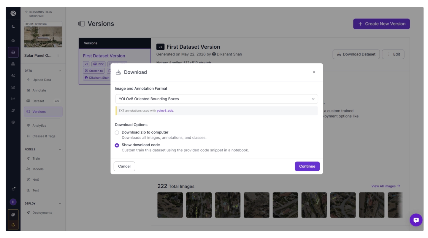
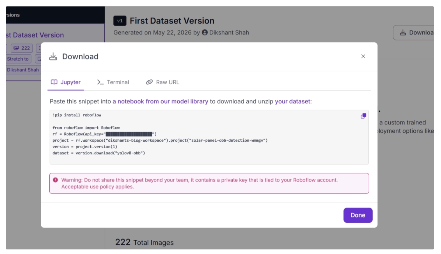
Within your project’s Versions menu, click “Download Dataset” and select “Show download code.” Then choose the image and annotation format as “YOLOv8 Oriented Bounding Boxes.” This format is also supported by YOLO26 for training OBB detection, as shown below.

Once you click Continue, a code snippet will appear that you can use to export your labeled dataset and download it directly into Google Colab in YOLOv8-OBB format.

Step 6: Download the dataset in Google Colab

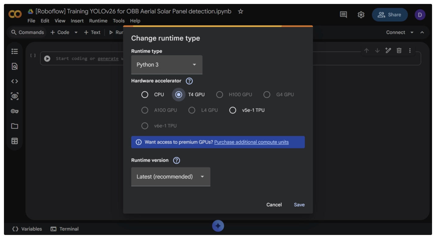
Now go to Google Colab and create a new notebook. Since YOLO26 requires a GPU, ensure the runtime is set to a T4 GPU by selecting it in the runtime settings as shown below and saving it.

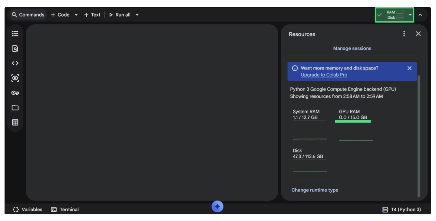
You can verify this by clicking the “RAM | Disk” indicator in the top-right corner. This will open a panel displaying available Colab resources, including system RAM, disk usage, and GPU memory, as shown below.

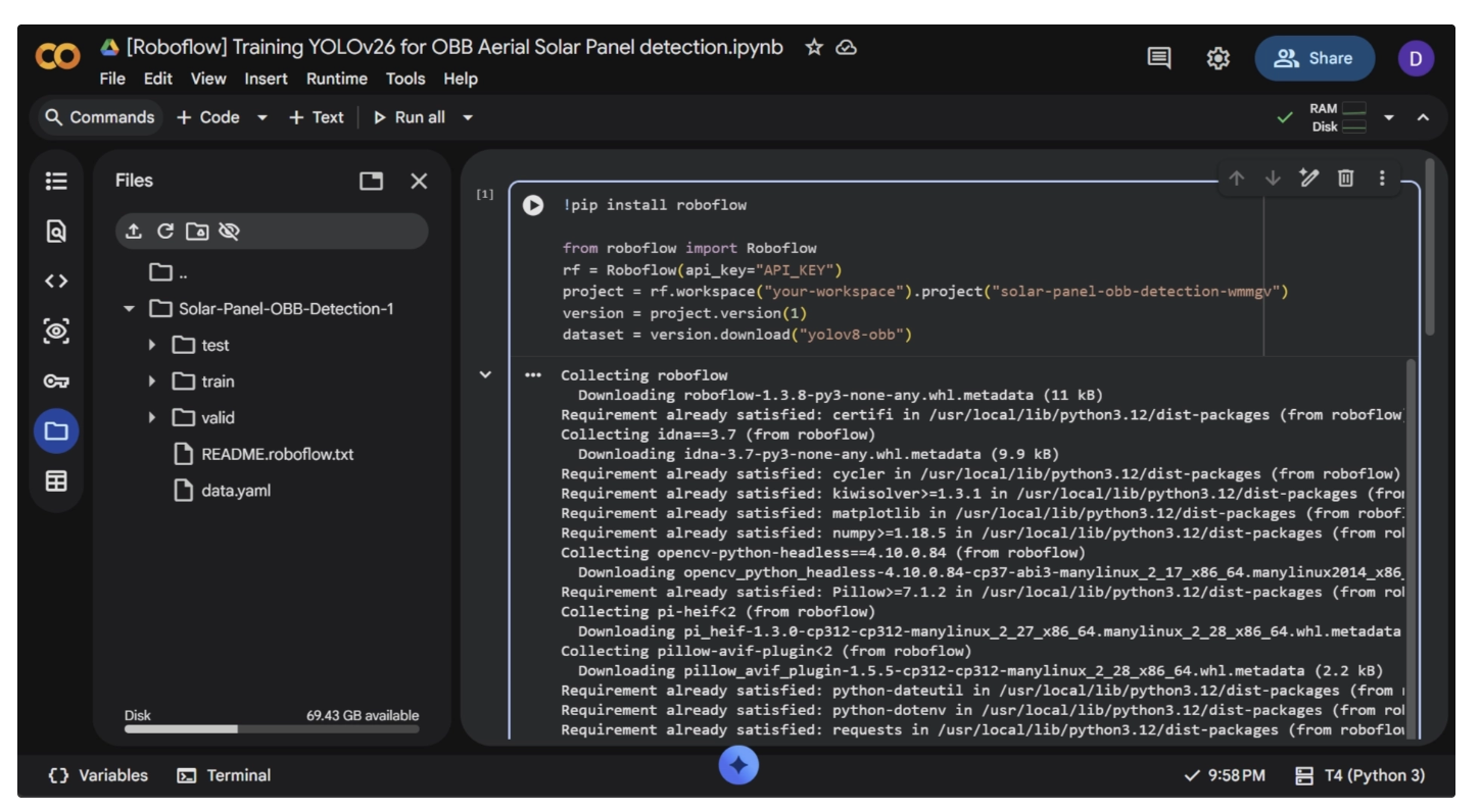
Then run the code snippet shown below, which was previously provided by Roboflow to export and download the dataset directly into Google Colab in YOLOv8-OBB format.

Your API key, workspace name, and project ID will be automatically filled in when you copy the snippet directly from Roboflow.

!pip install roboflow

from roboflow import Roboflow
rf = Roboflow(api_key="API_KEY")
project = rf.workspace("your-workspace").project("solar-panel-obb-detection-wmmgv")
version = project.version(1) # Dataset Version
dataset = version.download("yolov8-obb")

When you run this code snippet, it downloads the dataset in YOLOv8-OBB format, which is a supported format for training YOLO26 for oriented bounding box detection.

Once the execution is complete, you can see the dataset appear in the left navigation panel.

Step 7: Train a YOLO26 OBB Model

Now that we have downloaded the dataset, we can train a YOLO26-OBB model. To use YOLO models, you need to install the package. You can do this by running the code snippet below:

# install the Ultralytics package quietly (-q hides detailed installation logs)
!pip install ultralytics -q

# disable Ultralytics analytics/tracking sync
!yolo settings sync=False

# import the ultralytics library
import ultralytics

# run environment and dependency checks
# this displays information such as Python version, PyTorch version, CUDA availability, GPU info, etc.
ultralytics.checks()

Next, we need to set up the pretrained YOLO model that we will use as the starting point. This allows us to leverage existing learned features instead of training from scratch.

# import the YOLO class from the Ultralytics library
from ultralytics import YOLO

# load the pretrained YOLO26 nano OBB (Oriented Bounding Box) model
# the .pt file contains the pretrained model weights
model = YOLO('yolo26n-obb.pt')

After that, we update the dataset configuration file so that YOLO can correctly locate the training, validation, and testing images. This helps avoid path-related errors during training.

import yaml  # used to read and write YAML files

# open the dataset configuration file (data.yaml)
with open(f'{dataset.location}/data.yaml', 'r') as f:
    data = yaml.safe_load(f)  # load YAML content into a Python dictionary

# update dataset paths for training, validation, and testing images
data['train'] = '../train/images'
data['val'] = '../valid/images'
data['test'] = '../test/images'

# remove 'path' key if it exists (avoids conflicts in YOLO training configs)
if 'path' in data:
    del data['path']

# write the updated configuration back to the same YAML file
with open(f'{dataset.location}/data.yaml', 'w') as f:
    yaml.dump(data, f, sort_keys=False)  # save YAML without sorting keys

Finally, we begin training the YOLO26-OBB model using our prepared dataset by specifying the number of training epochs and image size.

The ‘epochs’ parameter controls how long the model trains, while ‘imgsz’ defines the input image resolution used during training. Make sure the resolution used in your dataset preprocessing matches the value provided in the ‘imgsz’ parameter for consistent training results.

Run the command:

results = model.train(data=f"{dataset.location}/data.yaml", epochs=100, imgsz=640)

The amount of time training takes will depend on the hardware on which you are running and how many images are in your dataset. Ours took 9.66 minutes on Google Colab with T4 GPU.

Step 8: Evaluate the Model on Test Images

Now that the model has been trained, we can load the best-performing weights saved during training and use them to test how well the model performs on unseen images from the test dataset.

The below code loads the trained OBB model:

# load the trained YOLO OBB model from the best saved weights after training
model = YOLO('runs/obb/train/weights/best.pt')

Then, define the path to the test images:

import os

# path to test images
test_dir = f"{dataset.location}/test/images"

# get all image files
image_files = [
    os.path.join(test_dir, f)
    for f in os.listdir(test_dir)
]

Now, run Inference and visualize predictions on all test Images:

# supervision is a python library used for visualizion
!pip install supervision -q

import supervision as sv
import cv2

# loop through all test images
for file_name in image_files:

    # run inference
    results = model(file_name)

    # convert to supervision format
    detections = sv.Detections.from_ultralytics(results[0])

    # create confidence labels (whole number % only)
    labels = [
        f"{int(conf * 100)}%"
        for conf in detections.confidence
    ]

    # annotators
    oriented_box_annotator = sv.OrientedBoxAnnotator()

    label_annotator = sv.LabelAnnotator(
        text_scale=0.3,
        text_padding=2
    )

    # read image
    image = cv2.imread(file_name)

    # draw boxes
    annotated = oriented_box_annotator.annotate(
        scene=image,
        detections=detections
    )

    # draw labels
    annotated = label_annotator.annotate(
        scene=annotated,
        detections=detections,
        labels=labels
    )

    # resize for display
    annotated = sv.resize_image(
        annotated,
        resolution_wh=(900, 900),
        keep_aspect_ratio=True
    )

    # display
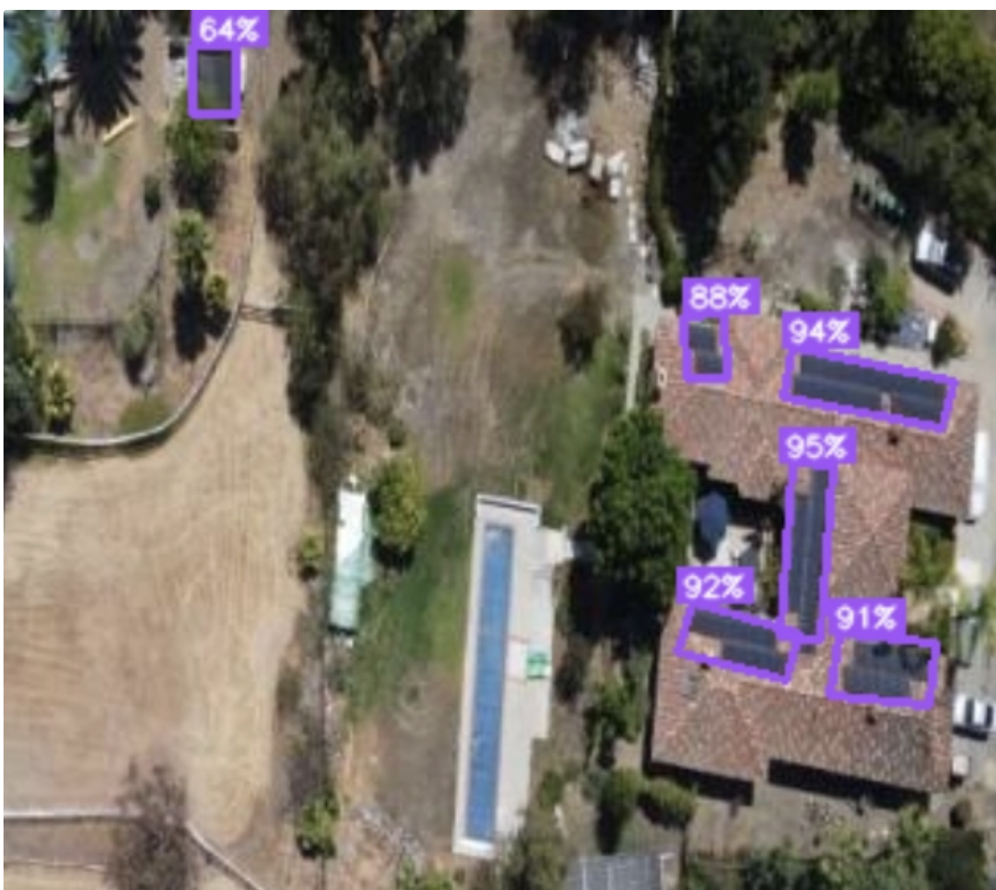
    display(sv.cv2_to_pillow(annotated))

One of the resulting visualizations on a test image is shown below, where the model successfully detects solar panels, predicts their orientation, and provides the corresponding confidence scores.

Conclusion: Training YOLO26 Oriented Bounding Box (OBB) Model

Oriented Bounding Box (OBB) provides a more precise way to understand objects in real-world images by capturing both their position and orientation.

This is especially useful for aerial imagery analysis, where objects are often rotated, densely packed, or not aligned with the image frame. In such cases, standard bounding boxes can include unnecessary background, while OBBs fit the object more closely and improve localization accuracy.

In this guide, we walked through training a YOLO26-OBB model, starting from dataset preparation and exporting annotations in OBB format, and continuing through to training and evaluating the model.

Roboflow simplified the entire training process by enabling dataset versioning and offering preprocessing tools to effectively prepare the data for training.

At the same time, Roboflow Annotate accelerated the labeling process for aerial imagery through intuitive polygon tools and AI-assisted annotation features.

You can try Roboflow now for free to easily train models for a wide range of computer vision tasks.

Cite this Post

Use the following entry to cite this post in your research:

James Gallagher. (May 1, 2026). How to Train a YOLO26 Oriented Bounding Box (OBB) Model. Roboflow Blog: https://blog.roboflow.com/train-yolov8-obb-model/