
EfficientNet is a convolutional neural network architecture introduced by Google AI in 2019 that scales width, depth, and input resolution together using a method called compound scaling. By tuning all three dimensions proportionally rather than independently, EfficientNet achieves strong accuracy with far fewer parameters than prior architectures: the top variant matches GPipe on ImageNet using 66 million parameters versus 556 million. The architecture also uses Mobile Inverted Bottleneck layers and Squeeze-and-Excitation blocks to stay efficient across varying hardware budgets.
Introduced in 2019 by a team of researchers at Google AI, EfficientNet became a go-to architecture for many challenging tasks, including object recognition, image segmentation, and even language processing. Its success stems from its ability to balance two critical factors in deep learning: computational efficiency and model performance.
Traditional deep learning models often come with a trade-off between accuracy and resource consumption. EfficientNet addresses this challenge by introducing a novel approach called "compound scaling."
By systematically scaling the model's dimensions (width, depth, and resolution) in a principled manner, EfficientNet achieves unprecedented levels of efficiency without compromising accuracy. This method allows the model to strike an optimal balance, making it adaptable to various computational budgets and hardware capabilities.
In this blog post, we will dive deep into the architecture of EfficientNet, explore the technical details behind compound scaling, and understand how compound scaling has transformed the field of deep learning.
Without further ado, let’s begin!
What is EfficientNet?
EfficientNet is a convolutional neural network built upon a concept called "compound scaling.” This concept addresses the longstanding trade-off between model size, accuracy, and computational efficiency. The idea behind compound scaling is to scale three essential dimensions of a neural network: width, depth, and resolution.
- Width: Width scaling refers to the number of channels in each layer of the neural network. By increasing the width, the model can capture more complex patterns and features, resulting in improved accuracy. Conversely, reducing the width leads to a more lightweight model, suitable for low-resource environments.
- Depth: Depth scaling pertains to the total number of layers in the network. Deeper models can capture more intricate representations of data, but they also demand more computational resources. On the other hand, shallower models are computationally efficient but may sacrifice accuracy.
- Resolution: Resolution scaling involves adjusting the input image's size. Higher-resolution images provide more detailed information, potentially leading to better performance. However, they also require more memory and computational power. Lower-resolution images, on the other hand, consume fewer resources but may lead to a loss in fine-grained details.
The figure below illustrates the impact of scaling means across different dimensions.
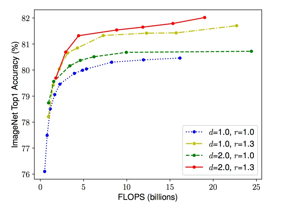
Scaling Network Width for Different Baseline Networks. Each dot in a line denotes a model with a different width coefficient (w). The first baseline network (d=1.0, r=1.0) has 18 convolutional layers with a resolution of 224x224, while the last baseline (d=2.0, r=1.3) has 36 layers with a resolution of 299x299. Source
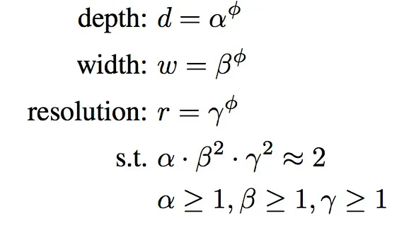
One of the strengths of EfficientNet lies in its ability to balance these three dimensions through a principled approach. Starting from a baseline model, the researchers perform a systematic grid search to find the optimal combination of width, depth, and resolution. This search is guided by a compound coefficient, denoted as "phi" (φ) which uniformly scales the dimensions of the model. This φ value acts as a user-defined parameter that determines the model's overall complexity and resource requirements.
Let’s walk through how compound scaling works step-by-step.
How Compound Scaling Works
The process begins with a baseline model, which serves as the starting point. This baseline model is usually a reasonably sized neural network that performs well on a given task but may not be optimized for computational efficiency.
Then, a compound coefficient is introduced as a user-defined parameter that dictates how much to scale the dimensions of the neural network. It is a single scalar value that uniformly scales the width, depth, and resolution of the model. By adjusting this φ value, the overall complexity and resource requirements of the model can be controlled.
From here, dimensions are scaled. The key idea behind compound scaling is to scale the dimensions of the baseline model (width, depth, and resolution) in a balanced and coordinated manner. The scaling factors for each dimension are derived from the compound coefficient φ.
- Width Scaling: The width of the neural network is scaled proportionally by raising φ to the power of a specific exponent (typically denoted as α).
- Depth Scaling: Similarly, the depth of the network is scaled by raising φ to another exponent (commonly denoted as β).
- Resolution Scaling: The resolution or input image size is scaled by multiplying the original resolution (r) by φ raised to a different exponent (usually denoted as γ).
Next, optimal exponents need to be determined. The exponents α, β, and γ are constants that need to be determined to achieve the most optimal scaling. The values of these exponents are typically derived through an empirical grid search or optimization process. The goal is to identify the combination of exponents that results in the best trade-off between model accuracy and computational efficiency.
Once the scaling factors for width, depth, and resolution are determined, they are applied to the baseline model accordingly. The resulting model is now the EfficientNet with a specific φ value.
Depending on the specific use case and available computational resources, researchers and practitioners can choose from a range of EfficientNet models, each corresponding to a different φ value. Smaller φ values lead to more lightweight and resource-efficient models, while larger φ values result in more powerful but computationally intensive models.
By following the compound scaling method, EfficientNet can efficiently explore a wide range of model architectures that strike the perfect balance between accuracy and resource consumption. This remarkable ability to scale effectively has made EfficientNet a game-changer in the field of deep learning, enabling state-of-the-art performance on various computer vision tasks while remaining adaptable to diverse hardware constraints.
EfficientNet Architecture
EfficientNet uses Mobile Inverted Bottleneck (MBConv) layers, which are a combination of depth-wise separable convolutions and inverted residual blocks. Additionally, the model architecture uses the Squeeze-and-Excitation (SE) optimization to further enhance the model's performance.
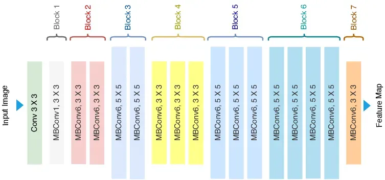
The MBConv layer is a fundamental building block of the EfficientNet architecture. It is inspired by the inverted residual blocks from MobileNetV2 but with some modifications.
The MBConv layer starts with a depth-wise convolution, followed by a point-wise convolution (1x1 convolution) that expands the number of channels, and finally, another 1x1 convolution that reduces the channels back to the original number. This bottleneck design allows the model to learn efficiently while maintaining a high degree of representational power.
In addition to MBConv layers, EfficientNet incorporates the SE block, which helps the model learn to focus on essential features and suppress less relevant ones. The SE block uses global average pooling to reduce the spatial dimensions of the feature map to a single channel, followed by two fully connected layers.
These layers allow the model to learn channel-wise feature dependencies and create attention weights that are multiplied with the original feature map, emphasizing important information.
EfficientNet comes in different variants, such as EfficientNet-B0, EfficientNet-B1, and so on, with varying scaling coefficients. Each variant represents a different trade-off between model size and accuracy, enabling users to select the appropriate model variant based on their specific requirements.
EfficientNet Performance
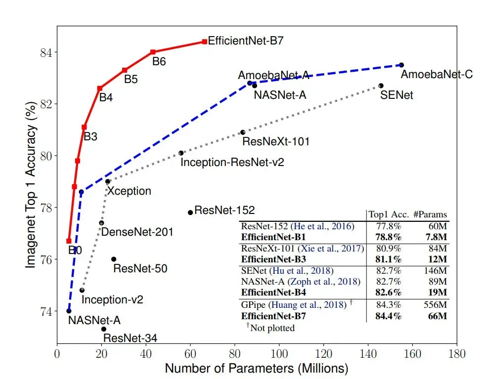
The figure above depicts the EfficientNet curve highlighted by a red line. On the horizontal axis lies the model size, while the vertical axis represents the accuracy rate. A mere glance at this illustration is enough to underscore the prowess of EfficientNet. In terms of accuracy, EfficientNet outshines its predecessors by a mere 0.1%, edging slightly past the former state-of-the-art model, GPipe.
What's notable is the method employed to achieve this accuracy. While GPipe relies on 556 million parameters, EfficientNet accomplishes the same with a mere 66 million - a huge contrast. In practical scenarios, the marginal 0.1% accuracy gain might go unnoticed. However, the remarkable eightfold increase in speed significantly enhances the network's usability and its potential for real-world industrial applications.
Conclusion
EfficientNet, with its compound scaling methodology, had an impact on our understanding of the balance between efficiency and accuracy in deep learning. By intelligently scaling width, depth, and resolution, it offers versatile models adaptable to various hardware constraints.
The architecture's lightweight and robust design, combined with Mobile Inverted Bottleneck layers and Squeeze-and-Excitation optimization, consistently delivers high performance across several computer vision tasks.
Cite this Post
Use the following entry to cite this post in your research:
Petru P.. (Aug 9, 2023). What is EfficientNet? The Ultimate Guide.. Roboflow Blog: https://blog.roboflow.com/what-is-efficientnet/