
Dimensionality reduction techniques compress high-dimensional datasets into lower-dimensional representations while preserving the structure and relationships that matter for analysis and modeling. This guide covers the three most widely used methods: PCA, which finds linear projections that maximize variance and works well for structured numeric data; t-SNE, which reveals local cluster structure but can distort global relationships; and UMAP, which offers faster computation and better preservation of both local and global structure. Choosing among them depends on data type, dataset size, and whether the goal is visualization, preprocessing, or exploratory analysis.
Introduction to Dimensionality Reduction
Dimensionality reduction, a critical technique in machine learning and data analysis, has seen considerable advancements in recent years, addressing the challenges posed by high-dimensional data in various fields. This technique, which involves reducing the number of input variables or features, is crucial for simplifying models, improving performance, and reducing computational costs while retaining essential information.
Dimensionality reduction techniques can transform complex datasets by mapping them into lower-dimensional spaces while preserving relationships within the data, such as patterns or clusters that are often obscured in high-dimensional environments.
This approach to simplifying data structures leads to more efficient algorithms, enables better visualization, and reduces the risk of overfitting in machine learning models. Dimensionality reduction is particularly effective in areas like image processing, natural language processing, and genomics, where the volume of features can be overwhelming.
In this blog post, we will explore the core techniques of dimensionality reduction, examine their applications, and discuss their impact on modern data science and machine learning workflows.
What is Dimensionality Reduction?
Dimensionality reduction is a key technique in data analysis and machine learning, designed to reduce the number of input variables or features in a dataset while preserving the most relevant information. In real-world datasets, the presence of numerous variables can increase complexity, make models prone to overfitting, and reduce interpretability.
Dimensionality reduction techniques tackle these challenges through the creation of new variables or projections that capture the data’s essential characteristics. The objective is to retain the underlying structure, patterns, and relationships within the data while working with fewer dimensions.
By reducing dimensionality, the data becomes easier to visualize, explore, and analyze, leading to faster computations, improved model performance, and clearer insights into the underlying factors driving the data.
Why is Dimensionality Reduction Necessary?
Dimensionality reduction necessary for several reasons, in particular:
Curse of Dimensionality: High-dimensional data often suffers from sparsity, making it difficult to gain useful insights or build accurate models. As the number of features increases, data points become spread out, reducing their density. Dimensionality reduction counters this issue by reducing feature space, improving the data’s density and interpretability.
Computational Efficiency: The more features a dataset contains, the more computationally expensive it becomes to run machine learning algorithms. Dimensionality reduction helps by lowering the number of features, reducing the computational burden, and enabling faster data processing and model training.
Overfitting Prevention: Datasets with too many features are more susceptible to overfitting, where models capture noise or random variations rather than the true patterns. By reducing the dimensionality, we minimize the risk of overfitting, leading to more robust and generalizable models.
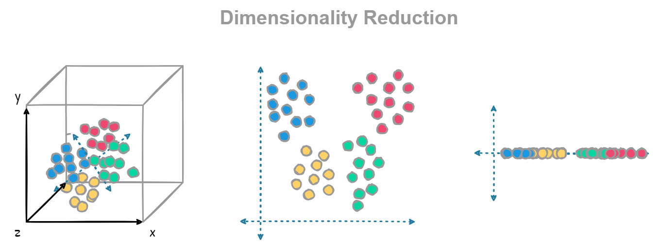
Visualization and Interpretation: Visualizing data in high dimensions (beyond three dimensions) is inherently difficult. Dimensionality reduction techniques project data into lower-dimensional spaces, making it easier to visualize, interpret, and identify patterns or relationships among variables, thus enhancing data understanding and decision-making.
Key Features of Dimensionality Reduction
Dimensionality reduction techniques offer several important advantages in the fields of data analysis and machine learning:
Feature Selection: These methods help identify and retain the most informative and relevant features from the original dataset. By eliminating redundant or irrelevant variables, dimensionality reduction highlights the subset of features that best represent the underlying patterns and relationships in the data.
Data Compression: Dimensionality reduction compresses data by transforming it into a lower-dimensional form. This condensed representation preserves as much of the critical information as possible while reducing the overall size of the dataset. It also helps reduce both storage demands and computational complexity.
Noise Reduction: High-dimensional datasets often include noisy or irrelevant features that can distort analysis and model performance. Dimensionality reduction minimizes the effect of this noise by filtering out unimportant variables, thereby improving the data’s signal-to-noise ratio and enhancing the quality of analysis.
Enhanced Visualization: Since humans can only visualize data in up to three dimensions, high-dimensional datasets are difficult to interpret. Dimensionality reduction projects data into lower dimensions, typically two or three, enabling easier visualization and interpretation of patterns, clusters, and relationships within the data.
Common Dimensionality Reduction Techniques
In this section, we will explore some of the most commonly used dimensionality reduction techniques. Each method offers unique approaches to simplifying high-dimensional data while retaining its essential features, making them valuable tools in various machine learning and data analysis tasks.
Principal Component Analysis (PCA)
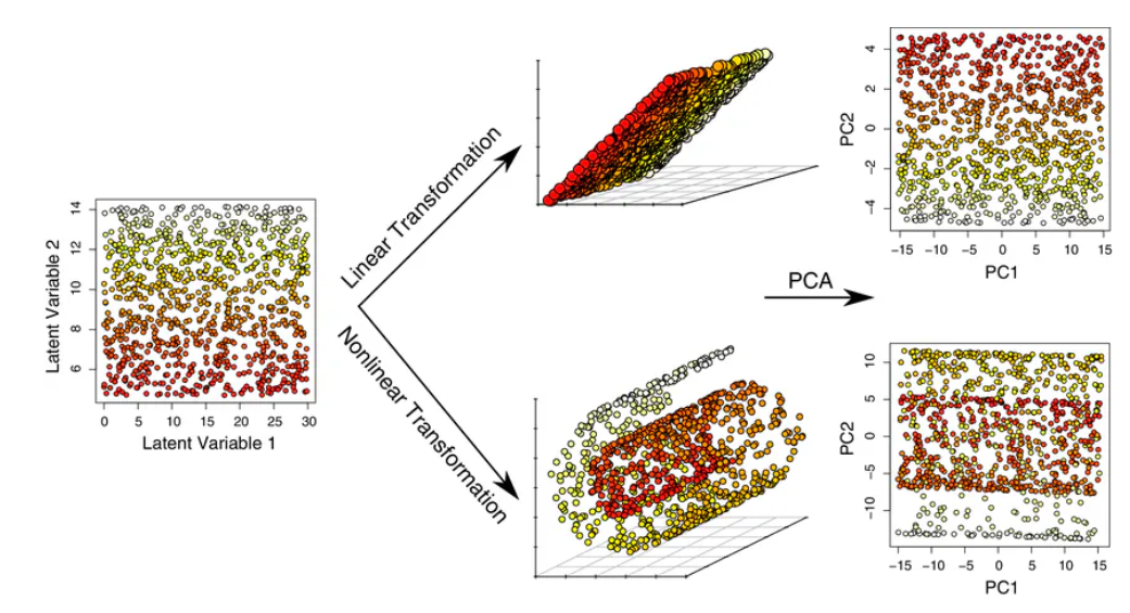
Principal Component Analysis (PCA) is a linear dimensionality reduction technique designed to extract a new set of variables from an existing high-dimensional dataset. Its primary goal is to reduce the dimensionality of the data while preserving as much variance as possible.
PCA is an unsupervised algorithm that creates linear combinations of the original features, known as principal components. These components are calculated such that the first one captures the maximum variance in the dataset, while each subsequent component explains the remaining variance without being correlated with the previous ones.
Rather than selecting a subset of the original features and discarding the rest, PCA forms new features through linear combinations of the existing ones, offering an alternative representation of the data. Often, only a few principal components are retained, the ones that are enough to capture around of the majority of the total variance. This is because each additional component explains progressively less variance and introduces more noise. By keeping fewer components, PCA effectively preserves the signal and filters out noise.
PCA improves interpretability while minimizing information loss, making it useful for identifying the most important features and for visualizing data in 2D or 3D. However, it is best suited for data with linear relationships and may struggle to capture complex patterns. Additionally, PCA is sensitive to significant outliers, which can distort the results.
t-Distributed Stochastic Neighbor Embedding (t-SNE)
t-SNE is a nonlinear dimensionality reduction algorithm designed for visualizing high-dimensional data. Its main goal is to maximize the probability of placing similar points close together in a low-dimensional space, while preserving the relationships between points that are farther apart as a secondary concern. It effectively clusters nearby points while pushing all other points apart.
Unlike PCA, t-SNE is a probabilistic technique. It minimizes the divergence between two distributions: one measuring pairwise similarities of the original data and another measuring similarities among the corresponding low-dimensional points. By aligning these distributions, t-SNE effectively represents the original dataset in fewer dimensions. Specifically, t-SNE employs a normal distribution for the high-dimensional space and a t-distribution for the low-dimensional space. The t-distribution is similar to the normal distribution but has heavier tails, allowing for a sparser clustering of points that enhances visualization.
t-SNE has several tunable hyperparameters, including:
Perplexity: This controls the size of the neighborhood for attracting data points.
Exaggeration: This adjusts the strength of attraction between points.
Learning Rate: This determines the step size for the gradient descent process that minimizes error.
Tuning these hyperparameters can significantly impact the quality and accuracy of t-SNE results. While t-SNE is powerful in revealing structures that other methods may miss, it can be difficult to interpret, as the original features become unidentifiable after processing. Additionally, because it is stochastic, different runs with varying initializations can produce different outcomes. Its computational and memory complexity is O(n²), which can demand substantial system resources.
Uniform Manifold Approximation and Projection (UMAP)
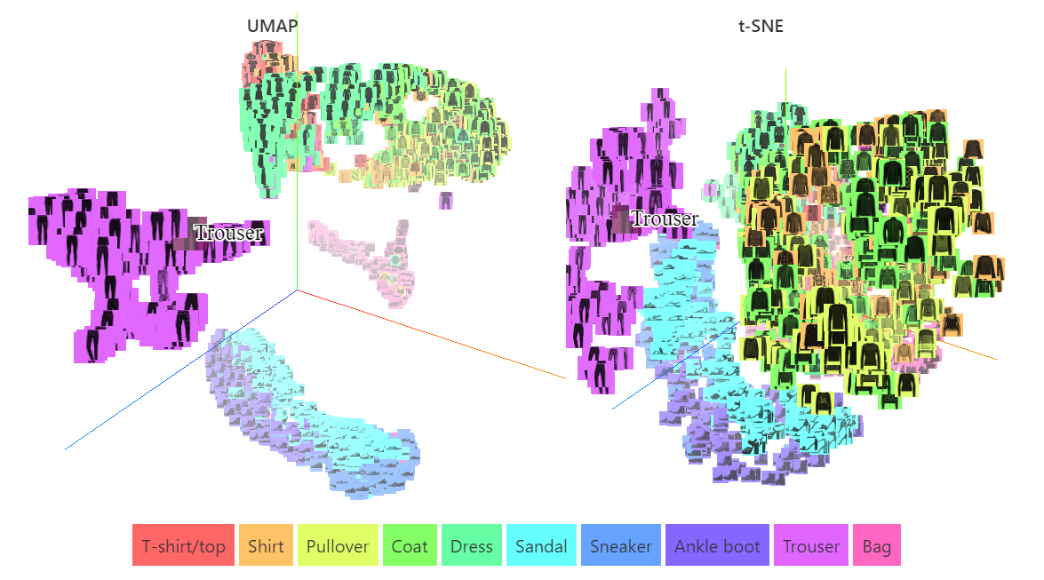
UMAP is a nonlinear dimensionality reduction algorithm that addresses some of the limitations of t-SNE. Like t-SNE, UMAP aims to create a low-dimensional representation that preserves relationships among neighboring points in high-dimensional space, but it does so with greater speed and better retention of the data’s global structure.
UMAP operates as a non-parametric algorithm in two main steps: (1) it computes a fuzzy topological representation of the dataset, and (2) it optimizes the low-dimensional representation to closely match this fuzzy topological representation, using cross-entropy as the measure. There are two key hyperparameters in UMAP that control the trade-off between local and global structures in the final output:
Number of Nearest Neighbors: This parameter determines the balance between local and global structure. Lower values focus on local details by limiting the number of neighboring points considered, while higher values emphasize the overall structure at the cost of finer details.
Minimum Distance: This parameter dictates how closely UMAP clusters data points in the low-dimensional space. Smaller values result in more tightly packed embeddings, whereas larger values lead to a looser arrangement, prioritizing the preservation of broader topological features.
Fine-tuning these hyperparameters can be complex, but UMAP's speed allows for multiple runs with different settings, enabling better insights into how projections vary.
When comparing UMAP to t-SNE, UMAP presents several notable advantages. Firstly, it delivers comparable visualization performance, allowing for effective representation of high-dimensional data. Additionally, UMAP excels in preserving the global structure of the data, ensuring that the distances between clusters are meaningful. This enhances interpretability and analysis of the relationships within the data.
Furthermore, UMAP operates with greater speed and efficiency, making it well-suited for handling large datasets without significant computational overhead. Finally, unlike t-SNE, which is primarily designed for visualization purposes, UMAP functions as a versatile dimensionality reduction tool that can be applied across various contexts and applications.
Conclusion
In summary, dimensionality reduction techniques such as PCA, t-SNE, and UMAP play a crucial role in data analysis and machine learning by simplifying complex, high-dimensional datasets. These methods not only help reduce computational costs and mitigate issues like overfitting but also enhance visualization and interpretability of data.
PCA is effective for linear data, providing a straightforward approach to identify the most important features while preserving variance. In contrast, t-SNE excels at revealing local structures in high-dimensional data, although it can struggle with global relationships and requires careful parameter tuning. UMAP addresses some of these limitations, offering faster performance and better preservation of global structure, making it suitable for a wider range of applications.
Ultimately, the choice of dimensionality reduction technique depends on the specific needs of your analysis, including the nature of the data, desired outcomes, and computational resources. By understanding the strengths and limitations of each method, you can effectively leverage these tools to gain deeper insights and drive informed decision-making in your projects.
Cite this Post
Use the following entry to cite this post in your research:
Petru P.. (Sep 27, 2024). What is Dimensionality Reduction? A Guide.. Roboflow Blog: https://blog.roboflow.com/what-is-dimensionality-reduction/