
Image embeddings let you measure similarity between images numerically, which makes them useful for assessing dataset quality, finding duplicates, and understanding class distribution without reviewing images by hand. This post demonstrates two approaches: clustering MNIST images using pixel brightness vectors reduced with t-SNE and UMAP, then applying OpenAI CLIP embeddings to a richer dataset to visualize class separation and retrieve visually similar images using cosine similarity. Together these techniques give computer vision practitioners practical tools for auditing and curating datasets before training.
Embeddings have become a hot topic in the field of natural language processing (NLP) and are gaining traction in computer vision. This blog post will explore the use of embeddings in computer vision by examining image clusters, assessing dataset quality, and identifying image duplicates.
We created a Google Colab notebook that you can run in a separate tab while reading this blog post, allowing you to experiment and explore the concepts discussed in real-time. Let’s dive in!
Clustering MNIST images using pixel brightness
Before we jump to examples involving OpenAI CLIP embeddings, let’s start with a less complex dataset— clustering MNIST images based on the brightness of their pixels.
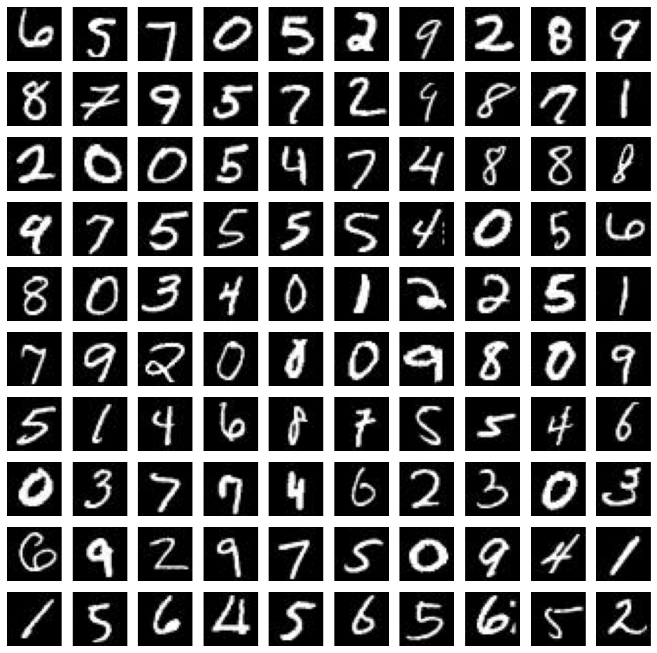
The MNIST dataset consists of 60,000 grayscale images of handwritten digits, each with a size of 28x28 pixels. Since each pixel in a grayscale image can be described by a single value, we have 784 values (or features) describing each image. Our goal is to use t-SNE and UMAP to reduce the number of dimensions to three, allowing us to display clusters of images in 3D space.
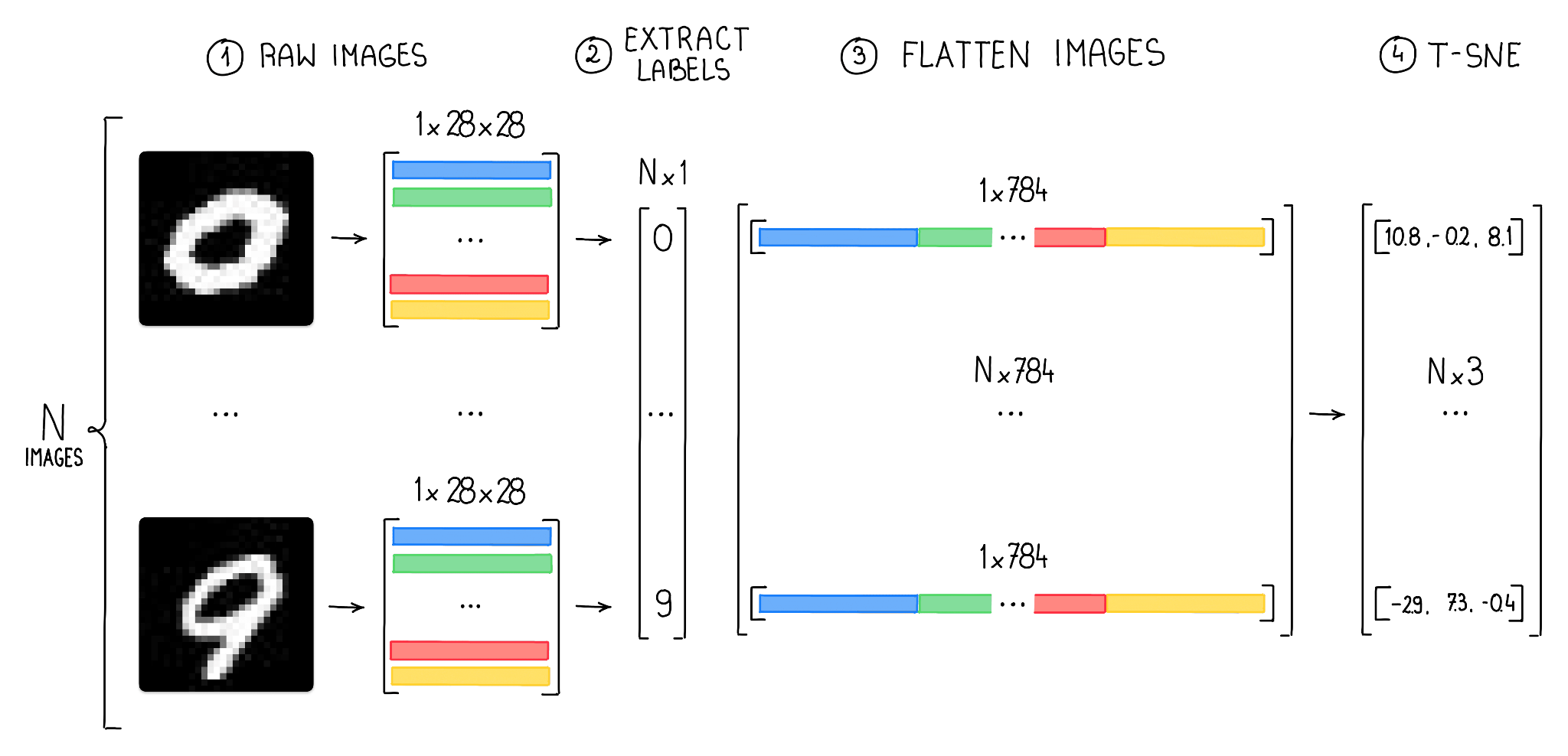
To accomplish this, we first need to load images of each class and reshape the data into a format that can be consumed by t-SNE (a 2D NumPy array with 784 features).
Visualizing High-dimensional Data
Visualizing and working with high-dimensional data can be challenging, as it becomes increasingly difficult to grasp the underlying structure and relationships in the data. Dimensionality reduction techniques, such as t-SNE and UMAP, are essential tools for simplifying these complex datasets, making them more manageable and easier to interpret.
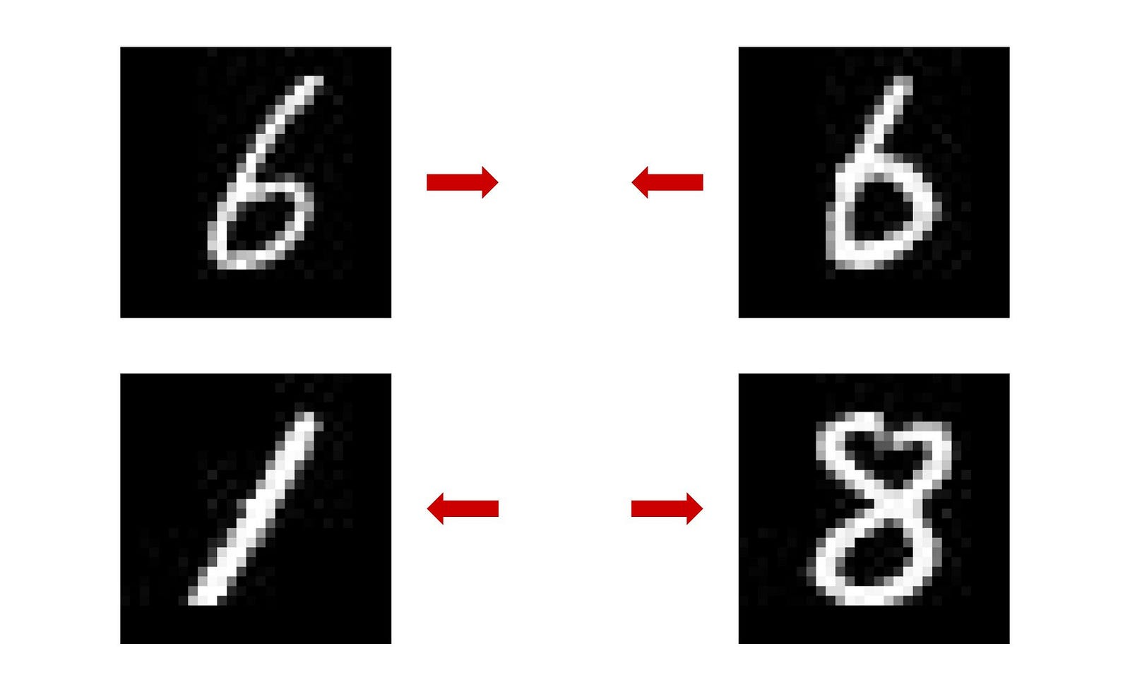
Two images depicting the number 6 in a similar writing style will be represented as points in a lower-dimensional space that are close to each other. This is because these techniques aim to preserve the relative similarity between data points in the original high-dimensional space. As a result, points representing similar images will be positioned near each other. Conversely, images showing different numbers, like 1 and 8, will be represented by points that are farther apart in the reduced-dimensional space.
t-SNE vs. UMAP
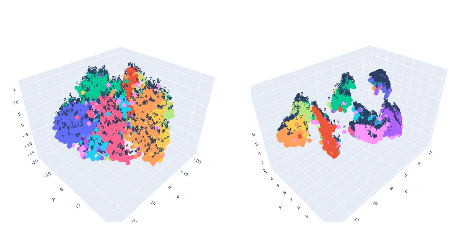
t-SNE and UMAP are both popular techniques for dimensionality reduction and visualization of high-dimensional data. However, there are some key differences between them. UMAP is known for its computational efficiency and scalability, which allows it to handle larger datasets more quickly compared to t-SNE. In our simple test using 5,000 images, UMAP was nearly 3x faster than t-SNE.
from sklearn.manifold import TSNE

projections = TSNE(n_components = 3).fit_transform(train)
from umap import UMAP
projections = umap.UMAP(n_components=3).fit_transform(train)Additionally, UMAP is designed to preserve the global structure better, while t-SNE primarily focuses on maintaining local relationships among data points. In practice, the choice between t-SNE and UMAP may depend on the specific needs and constraints of the task at hand, such as dataset size, computational resources, and the desired balance between local and global structure preservation.
Using OpenAI CLIP to Analyze Dataset Class Distribution
Pixel brightness is a suitable feature for the MNIST dataset because it comprises simple, grayscale images of handwritten digits, where the contrast between the digit and the background is the most crucial aspect. However, for regular images relying solely on pixel brightness is insufficient. These images have millions of pixels with varying color channels and contain much more complex and diverse visual information. Using pixel brightness as the primary feature in such cases would fail to capture the intricate details, textures, and relationships among objects in the image.
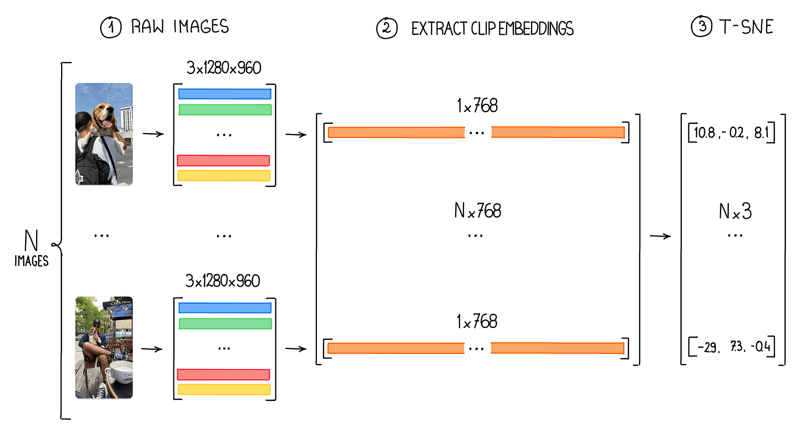
CLIP embeddings address this issue by providing a more abstract and compact representation of images, effectively encoding high-level visual and semantic information. These embeddings are generated by a powerful neural network trained on a diverse range of images, enabling it to learn meaningful features from complex, real-world photographs. By using CLIP embeddings, we can efficiently work with high-resolution images while preserving their essential visual and semantic characteristics for various computer vision tasks. You can get CLIP embeddings using the CLIP python package or directly from Roboflow search.
import clip

device = "cuda" if torch.cuda.is_available() else "cpu"
model, preprocess = clip.load("ViT-B/32", device=device)

image_path = "path/to/your/image.png"
image = preprocess(Image.open(image_path)).unsqueeze(0).to(device)

with torch.no_grad():
embeddings = model.encode_image(image)Identify Similar Images with Embeddings
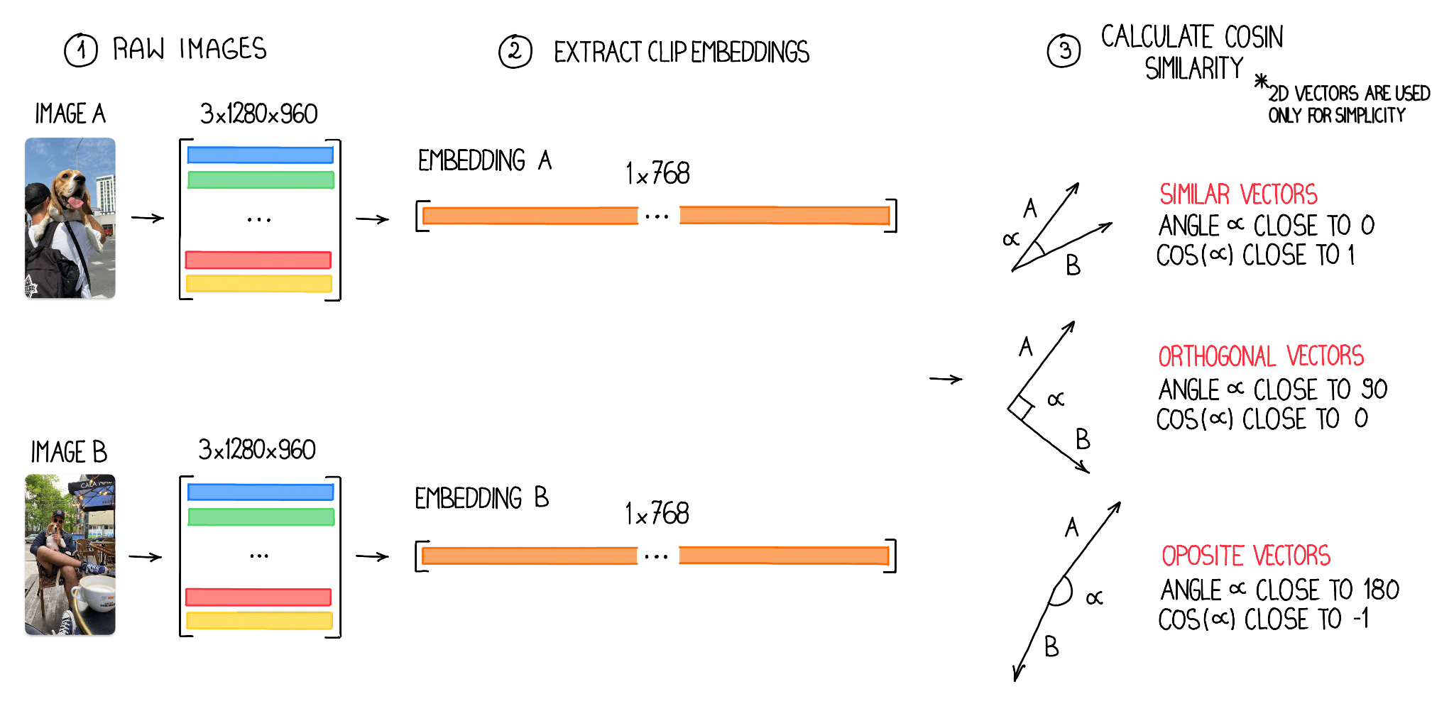
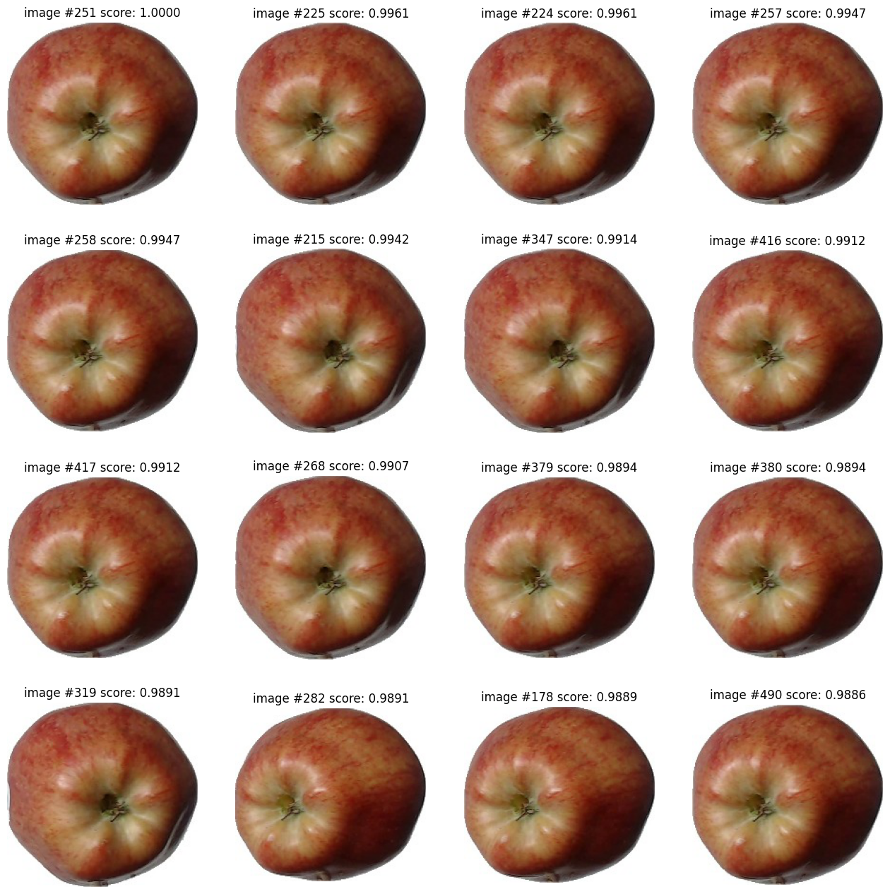
Embeddings can also be used to identify similar or close-to-similar images. By comparing the vectors of the embeddings, we can measure the similarity between two images using the cosine value. This value, which ranges from -1 to 1, provides a quantitative representation of image similarity. In the context of computer vision vector analysis, a cosine value of 1 indicates a high degree of similarity, a value of -1 indicates dissimilarity and a value of 0 suggests orthogonality, meaning the images share no common features. By leveraging this insight, we can effectively identify and group similar images based on their cosine values while distinguishing those that are unrelated or orthogonal.
In the process of searching for similar images, we first structure image embeddings into a 2D NumPy array with dimensions N x M, where N represents the number of analyzed images and M signifies the size of individual embedding vectors — in our case 768. Before computing the cosine similarity, it is essential to normalize these vectors.
Vector normalization is the process of scaling a vector to have a unit length, which ensures that the cosine similarity measures only the angular distance between vectors and not their magnitudes. With the normalized vectors, we can efficiently calculate the cosine similarity for all image pairs using vectorization, enabling us to identify and group similar images effectively.
Conclusion
OpenAI CLIP embeddings are an incredibly powerful tool in your Computer Vision arsenal. As we move forward, we plan to explore more use cases, test new models (other than CLIP), and delve deeper into the world of embeddings to help you unlock even more possibilities in the fast-paced field of computer vision. Stay tuned for future posts where we’ll continue to push the boundaries and unveil new ways to harness the power of embeddings.
Cite this Post
Use the following entry to cite this post in your research:
Piotr Skalski. (May 1, 2023). Leveraging Embeddings and Clustering Techniques in Computer Vision. Roboflow Blog: https://blog.roboflow.com/embeddings-clustering-computer-vision-clip-umap/