How to Fine-Tune SAM-2.1 on a Custom Dataset

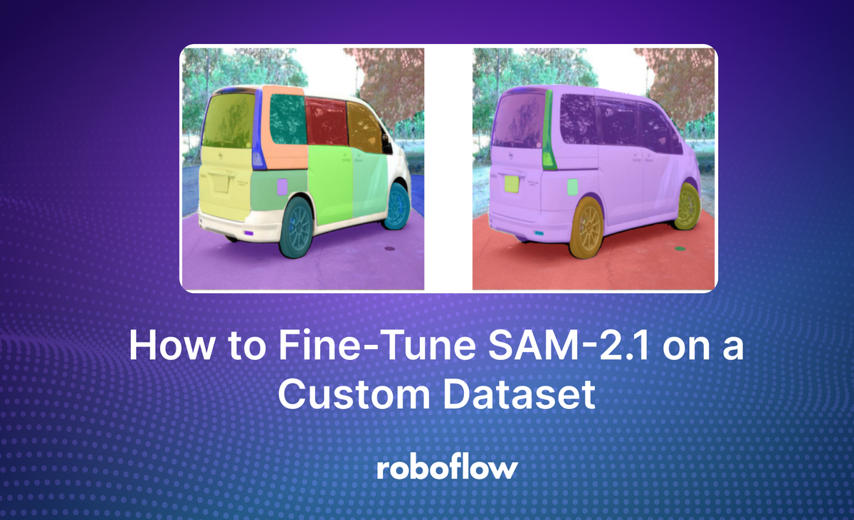
Released in September 2024 by Meta Research, SAM-2.1 is the latest model in the Segment Anything model series. When evaluated against the Segment Anything V test set, the MOSE validation set, and the LVOSv2 dataset, all SAM-2.1 model sizes perform better than SAM-2.

In this guide, we are going to walk through how to fine-tune SAM-2.1 on a custom dataset.

SAM-2.1 was released with training instructions that you can use to fine-tune SAM-2.1 for a specific use case. For instance, SAM-2.1 struggles to segment specific parts of a car (i.e. individual doors, windows). You could fine-tune SAM-2.1 to be able to identify and segment these parts.

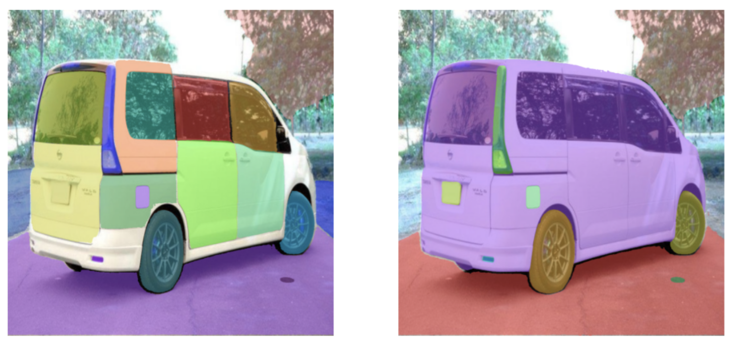
Below is a side-by-side comparison of SAM-2.1 segmenting car parts. On the left are the results from a fine-tuned SAM-2.1 model trained on segmenting car parts. On the right are the results from the out-of-the-box, base model. The results from the fine-tuned model are more precise than that of the base model.

Without further ado, let’s get started!

Step #1: Prepare Dataset

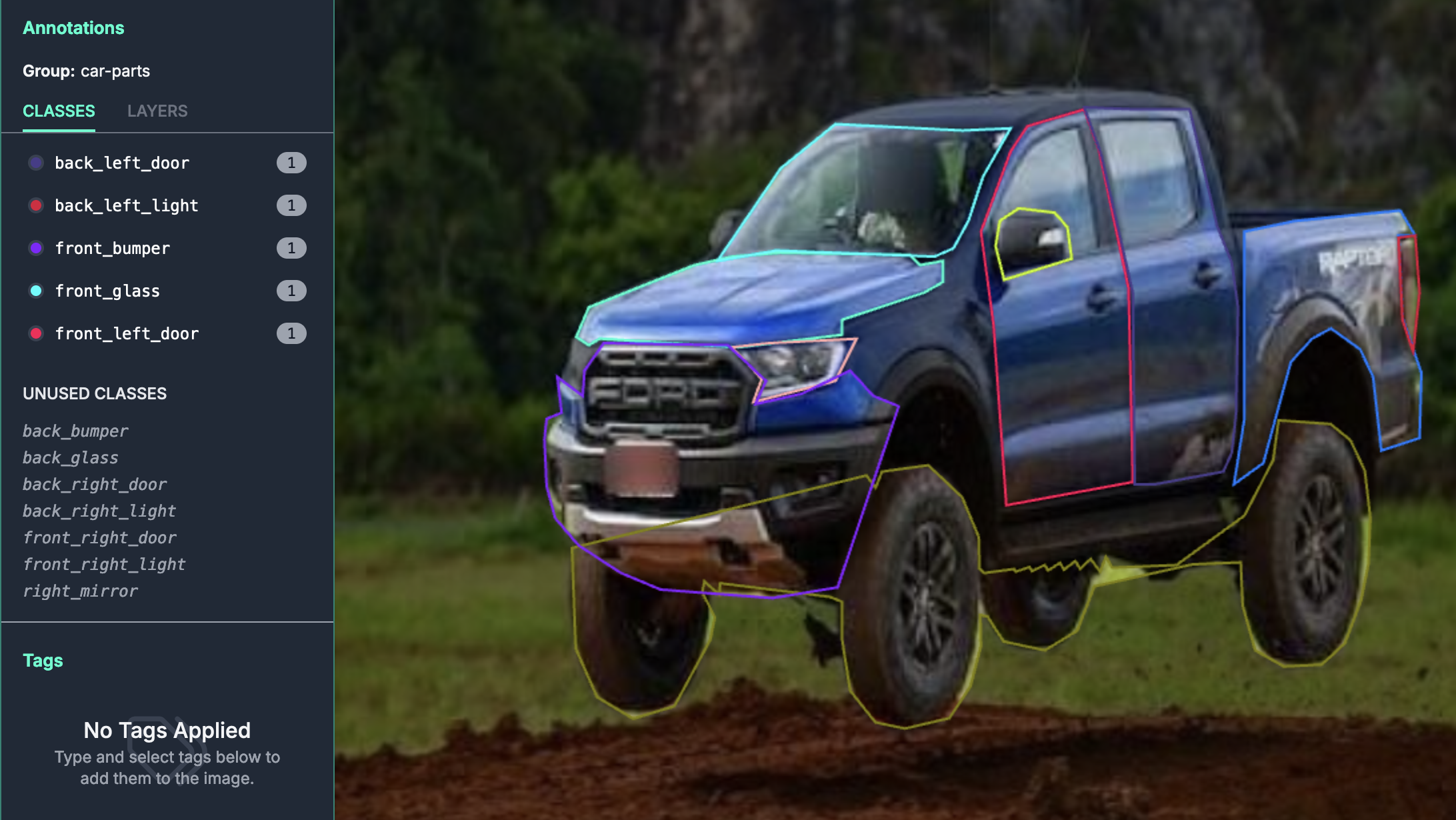
To get started, you will need a segmentation dataset with annotations. In this guide, we will be using the car parts dataset on Roboflow Universe. You can use Roboflow to create a dataset for your use case. To learn how to create a dataset in Roboflow, refer to the Roboflow Getting Started guide.

Here is an example of an annotation in our dataset, where each car part (i.e. back left door, back left light, front bumper) has its own label:

Once you have labeled your data, you are ready to generate a dataset.

You can generate SAM-2.1 datasets in Roboflow.

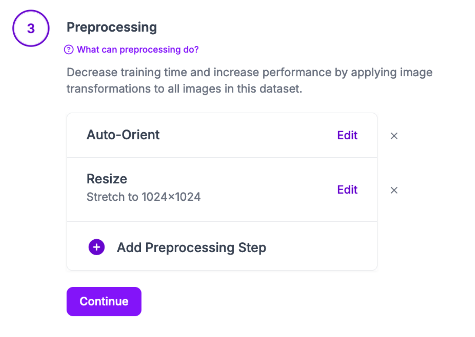
To do so, navigate to the Versions tab in your Roboflow project and click "Create New Version".

When you have generated a dataset in Roboflow, click “Export Dataset” on your dataset page:

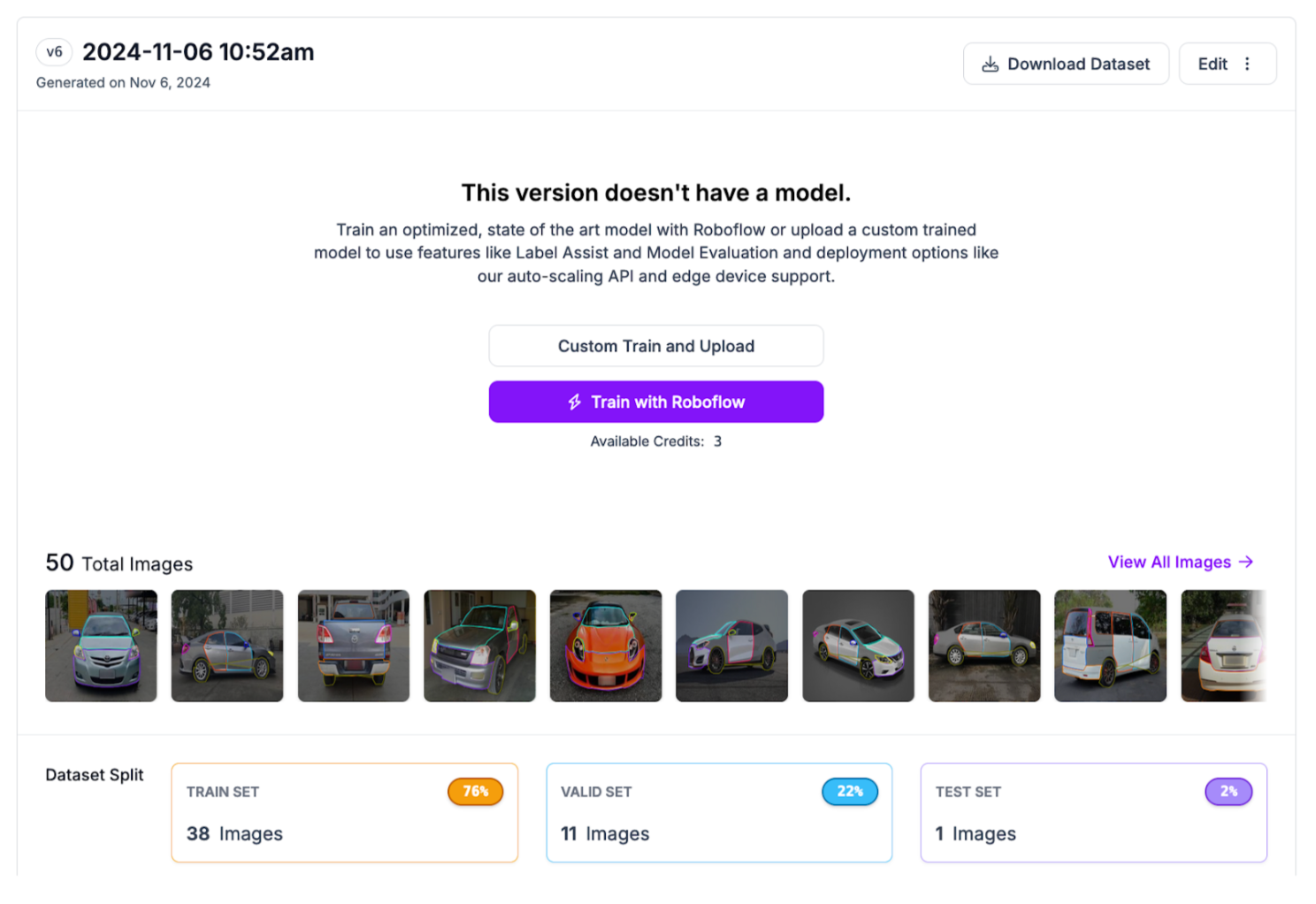
Select the SAM-2 export format:

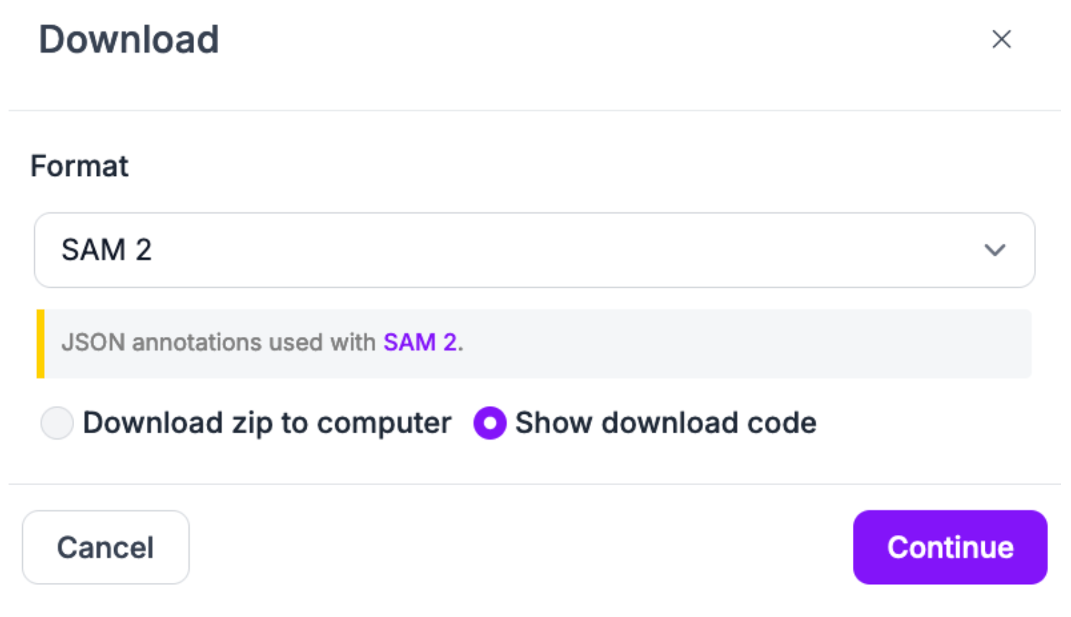
Copy the Jupyter Notebook download code. It will look something like this:

!pip install roboflow

from roboflow import Roboflow
rf = Roboflow(api_key="YOUR_KEY")
project = rf.workspace("brad-dwyer").project("car-parts-pgo19")
version = project.version(6)
dataset = version.download("sam2")

If you want to use our car parts dataset, you can use the above code snippet. You will need to add your Roboflow API key.

Step #2: Download SAM-2.1, Dataset, and Checkpoints

We have created a Colab notebook that walks through how to fine-tune SAM-2.1 on a custom dataset. We recommend opening the Colab notebook in a new tab as you follow along with this tutorial.

For optimal training speeds, we recommend training on an A100 in Colab if one is available. You can train a model on a T4, except the training times will be noticeably slower than they would be on an A100.

Once you have set up a notebook, first copy your dataset export code and run it.

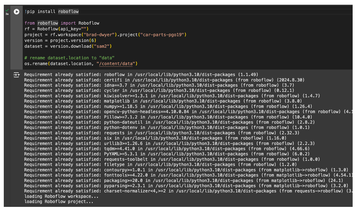
Then, rename the dataset folder to data:

import os

os.rename(dataset.location, "/content/data")

Then, download SAM-2.1 and our custom SAM-2.1 training YAML file:

!git clone https://github.com/facebookresearch/sam2.git
!wget -O /content/sam2/sam2/configs/train.yaml 'https://drive.usercontent.google.com/download?id=11cmbxPPsYqFyWq87tmLgBAQ6OZgEhPG3'

We can then navigate to the sam2 directory and install the model as well as supervision, a Python package for working with model predictions:

%cd ./sam2/
!pip install -e .[dev]
!pip install supervision -q

This step may take several minutes.

Next, we need to download the model checkpoints from which we can train a SAM-2.1 model.

The SAM-2.1 repository contains a script for downloading model checkpoints. You can download the checkpoints with the following command:

!cd ./checkpoints && ./download_ckpts.sh

Finally, we need to prepare our dataset for training. This involves modifying the file names in our dataset to ensure that they don’t contain various characters that we have found cause problems in the data loading stage. Run the following code to modify the file names in your training dataset as required:

import os
import re

FOLDER = "/content/data/train"

for filename in os.listdir(FOLDER):
	# Replace all except last dot with underscore
	new_filename = filename.replace(".", "_", filename.count(".") - 1)
	if not re.search(r"_\d+\.\w+$", new_filename):
    	# Add an int to the end of base name
    	new_filename = new_filename.replace(".", "_1.")
	os.rename(os.path.join(FOLDER, filename), os.path.join(FOLDER, new_filename))

Step #3: Start Training

Once you have prepared your dataset, installed SAM-2.1, and downloaded the model checkpoints, you are ready to start training a model.

You can train SAM-2.1 on a single or multiple GPUs. Since we are using Colab in this guide, we will train on a single GPU.

Run the following command to start training the model:

!python training/train.py -c 'configs/train.yaml' --use-cluster 0 --num-gpus 1

The amount of time training will take will depend on:

1. The number of GPUs you have (which will be 1 if you are using Colab);
2. The size of your dataset, and;
3. The type of GPU you are using.

When you start training, you should first see a print out of the config YAML file, followed by regular reports of the epoch at which your model is training:

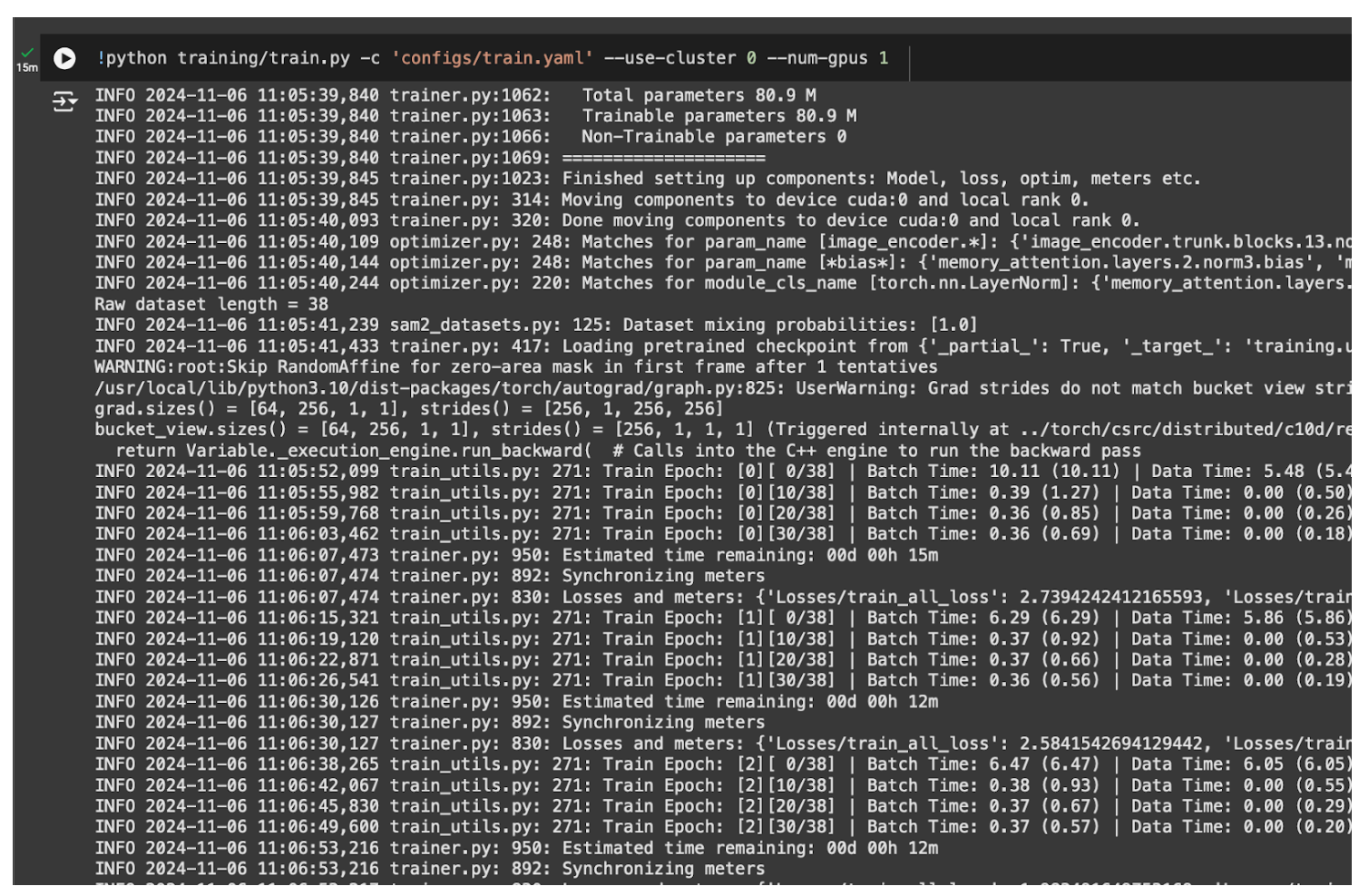
The amount of time it will take to fine-tune SAM depends on the number of images in your dataset, the number of epochs for which the model will train, and the GPU you are using.

Our training YAML sets the number of train epochs to 40.

For our car parts dataset with 38 training images, the model took 11 minutes to fine-tune.

Your model weights will be saved to:

/content/sam2/sam2_logs/configs/train.yaml/checkpoints/checkpoint.pt

You can view Tensorboard results from training with the following code in Colab:

%load_ext tensorboard
%tensorboard --bind_all --logdir ./sam2_logs/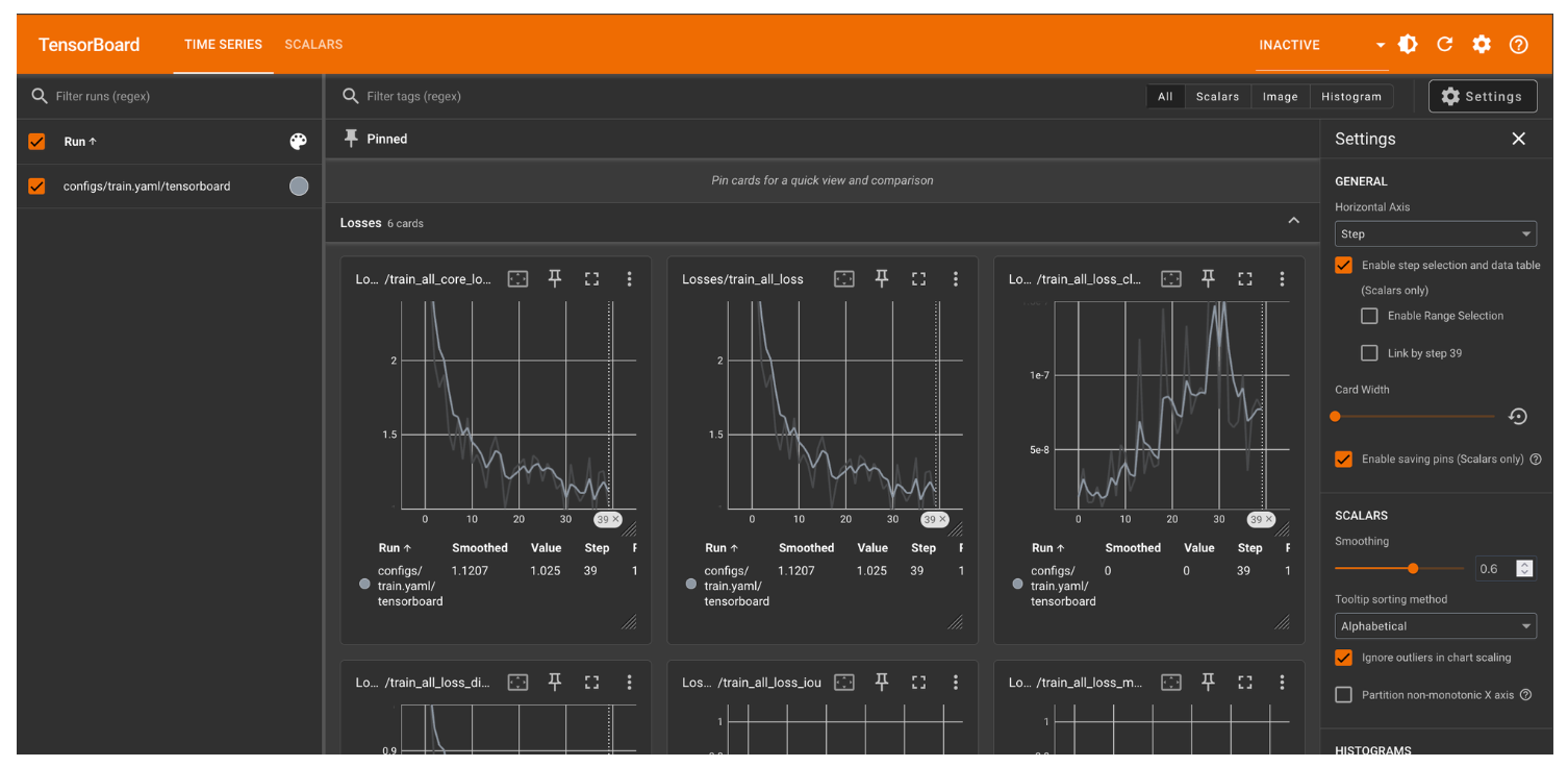

Step #4: Visualize Predictions

With a trained model ready, we can test the model on an image from our test set.

To assist with visualizing model predictions, we are going to use Roboflow supervision, an open source computer vision Python package with utilities for working with vision model outputs.

To install supervision, run:

pip install supervision

Then, create a code cell and add the following code:

import torch
from sam2.build_sam import build_sam2
from sam2.automatic_mask_generator import SAM2AutomaticMaskGenerator
import supervision as sv
import os
import random
from PIL import Image
import numpy as np

# use bfloat16 for inference
# from Meta notebook
torch.autocast("cuda", dtype=torch.bfloat16).__enter__()
if torch.cuda.get_device_properties(0).major >= 8:
	torch.backends.cuda.matmul.allow_tf32 = True
	torch.backends.cudnn.allow_tf32 = True

checkpoint = "/content/sam2/sam2_logs/configs/train.yaml/checkpoints/checkpoint.pt"
model_cfg = "configs/sam2.1/sam2.1_hiera_b+.yaml"
sam2 = build_sam2(model_cfg, checkpoint, device="cuda")
mask_generator = SAM2AutomaticMaskGenerator(sam2)

checkpoint_base = "/content/sam2/checkpoints/sam2.1_hiera_base_plus.pt"
model_cfg_base = "configs/sam2.1/sam2.1_hiera_b+.yaml"
sam2_base = build_sam2(model_cfg_base, checkpoint_base, device="cuda")
mask_generator_base = SAM2AutomaticMaskGenerator(sam2_base)

This will load our SAM-2.1 fine-tuned weights into the mask_generator variable and the base weights into the mask_generator_base variable.

We can then run inference on a random image in our validation set on both the base and fine-tuned models to evaluate model performance:

validation_set = os.listdir("/content/data/valid")

# choose random with .json extension
image = random.choice([img for img in validation_set if img.endswith(".jpg")])
image = os.path.join("/content/data/valid", image)
opened_image = np.array(Image.open(image).convert("RGB"))
result = mask_generator.generate(opened_image)

detections = sv.Detections.from_sam(sam_result=result)

mask_annotator = sv.MaskAnnotator(color_lookup = sv.ColorLookup.INDEX)
annotated_image = opened_image.copy()
annotated_image = mask_annotator.annotate(annotated_image, detections=detections)

base_annotator = sv.MaskAnnotator(color_lookup = sv.ColorLookup.INDEX)

base_result = mask_generator_base.generate(opened_image)
base_detections = sv.Detections.from_sam(sam_result=base_result)
base_annotated_image = opened_image.copy()
base_annotated_image = base_annotator.annotate(base_annotated_image, detections=base_detections)

sv.plot_images_grid(images=[annotated_image, base_annotated_image], grid_size=(1, 2))

Our code returns:

Our fine-tuned SAM-2.1 model (left) successfully segmented the objects in our image more precisely than the base model (right).

You can modify the code snippet below to use any of the prompting strategies supported by SAM-2.1, including calculating a segmentation mask for a region in a bounding box.

To learn more about SAM-2.1 prompting strategies, refer to the Meta SAM-2.1 inference notebooks.

Conclusion

You can fine-tune SAM-2.1 on a custom dataset. This is ideal if you plan to use SAM-2.1 in production and need to improve the model’s performance on a specific domain.

In this guide, we walked through how to fine-tune SAM-2.1. We prepared a segmentation dataset in Roboflow then exported the dataset for use in a Colab notebook. We then downloaded and set up SAM-2.1 and started training a model for 40 epochs.

Finally, we used supervision to visualize the output from the model.

To learn more about SAM-2.1’s capabilities, refer to the SAM-2 repository on GitHub. Meta has updated the repository to include information about SAM-2.1, including detailed accuracy metrics as evaluated against several large segmentation benchmarks.

Cite this Post

Use the following entry to cite this post in your research:

James Gallagher. (Nov 13, 2024). How to Fine-Tune SAM-2.1 on a Custom Dataset. Roboflow Blog: https://blog.roboflow.com/fine-tune-sam-2-1/

Discuss this Post

If you have any questions about this blog post, start a discussion on the Roboflow Forum.