
An autoencoder is a neural network that compresses an input into a compact latent vector and then reconstructs it, with the latent representation, not the output, being the useful artifact. Six main variants exist for computer vision: undercomplete, denoising, sparse, contrastive, Variational (VAE), and Vector Quantised-Variational (VQ-VAE), each suited to different tasks. In practice, autoencoders are applied to anomaly detection, semantic segmentation, super-resolution, and synthetic data generation, giving engineers a flexible unsupervised tool for extracting structured representations from image data.
In this blog post, we are going to introduce autoencoders, describe the several autoencoder types that exist, and showcase their applications.
An autoencoder is an artificial neural network used to learn data encodings in an unsupervised manner.
In other words, the autoencoder has to look at the data and construct a function that can transform a particular instance of that data into a meaningful representation.
Maybe this does not tell you much. Let's try to understand what this means and why we need it.
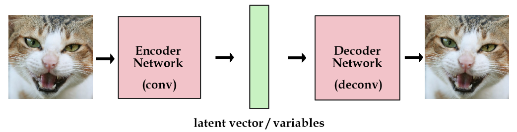
Consider the below architecture:
What is an Autoencoder?
Autoencoders have two main components: an encoder and a decoder. The encoder takes an input sample (the left cat image) and converts the information into some vector (the green block) which is essentially a set of numbers. We call this vector latent vector.
Then we have the decoder which takes this latent vector of numbers and expands it out to reconstruct the input sample.
Now, you may be wondering, why are we doing this? What is the point of trying to generate an output that is the same as the input?
And the answer to that is: well, there is no point.
When we use autoencoders, we actually do not care about the output itself, but rather we care about the vector constructed in the middle (the latent vector).
This vector is important because it is a representation of the input image and with this representation, we could potentially do several tasks like reconstructing the original image.
We can think of the latent vector as a code for an image, which is where the terms encode/decode come from.
The Structure of a Computer Vision Autoencoder
Now we are going to show a general structure of how an autoencoder is made and then we will go on to describe each individual part.
The architecture as a whole looks something like this:
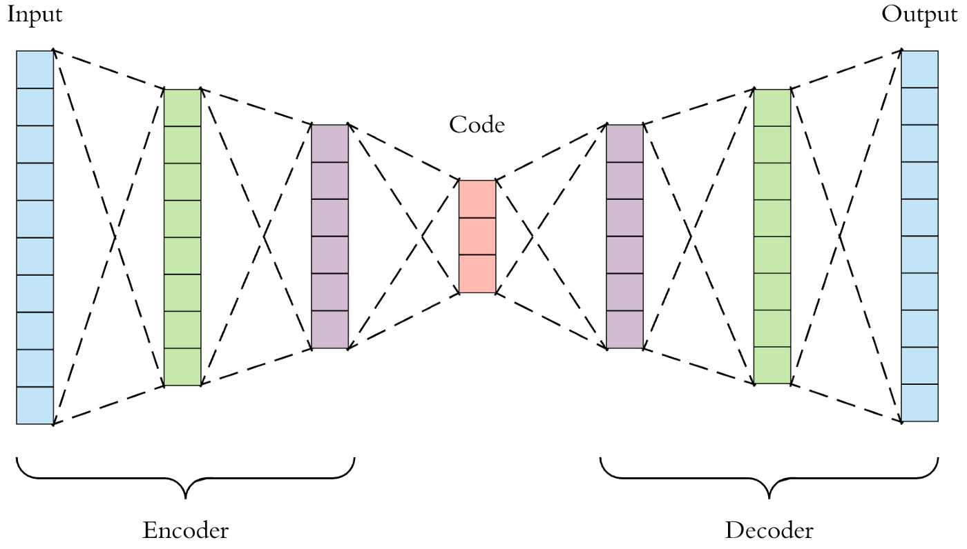
Autoencoders consist of 3 parts:
1. Encoder: a module that compresses the input data into an encoded representation that is typically several orders of magnitude smaller than the input data. The encoder is composed of a set of convolutional blocks followed by pooling modules or simple linear layers that compress the input to the model into a compact section called the "bottleneck" or "code".
2. Code: as you probably have already understood, the most important part of the neural network, and ironically the smallest one, is the code. The code exists to restrict the flow of information to the decoder from the encoder, thus, allowing only the most vital information to pass through. The code helps us form a knowledge representation of the input.
The code, as a compressed representation of the input, prevents the neural network from memorizing the input and overfitting the data. The smaller the code, the lower the risk of overfitting. This layer is generally implemented as a linear layer or as a tensor if we use convolutions.
3. Decoder: the decoder component of the network acts as an interpreter for the code.
The decoder helps the network to “decompress” the knowledge representations and reconstructs the data back from its encoded form. The output is then compared with the ground truth. This is usually implemented with transposed convolutions if we work with images or linear layers.
6 Types of Autoencoders for Computer Vision
The structure we have highlighted before is a general overview. Indeed, there exist several types of autoencoders. Here are the main autoencoders types to know:
Undercomplete Autoencoders
An Undercomplete Autoencoder takes an image as input and tries to predict the same image as output, thus reconstructing the image from the compressed code region. Undercomplete Autoencoders are unsupervised as they do not take any form of label in input as the target is the same as the input. The primary use of this type of autoencoder is to perform dimensionality reduction.
Why one should adopt autoecoders to perform dimensionality reduction instead of other methods like Principal Component Analysis (PCA)? Because PCA can only build linear relationships. Undercomplete Autoencoders can learn non-linear relationships and, therefore, perform better in dimensionality reduction.
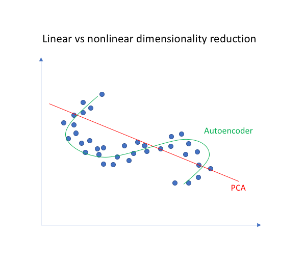
Effectively, if we remove all non-linear activations from an Undercomplete Autoencoder and use only linear layers, we reduce the autoencoder into something that works at an equal footing with PCA.
Denoising Autoencoders
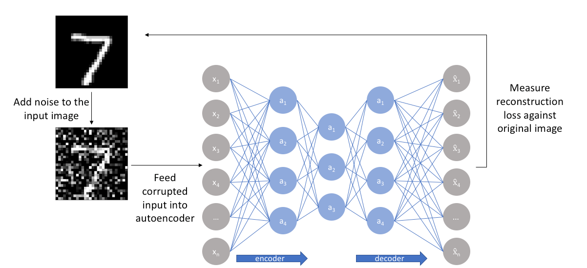
The aim of Denoising Autoencoders is to remove noise from an image.
How does this type of encoder achieve that? Instead of feeding the original image to the network as we would do normally, we create a copy of the input image, add artificial noise to it and feed this new noisy version of the image to the network. Then, the output is compared with the ground truth image.
In this way, the autoencoder gets rid of noise by learning a representation of the input where the noise can be filtered out easily. Below we show how the architecture of a Denoising Autoencoder is structured.
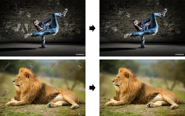
Another example where Denoising Autoencoders could be used is to remove the watermarks from an image. We show an example below.
Sparse AutoEncoders
This type of autoencoder explicitly penalizes the use of hidden node connections to prevent overfitting. How does it achieve this? We construct a loss function in order to penalize activations within a layer.
For any given observation, we encourage our network to learn an encoding and decoding that only relies on activating a small number of neurons. This is similar to dropout.
This allows the network to sensitize toward specific attributes of the input data. Whereas an Undercomplete Autoencoder will use the entire network for every observation, a Sparse Autoencoder will be forced to selectively activate regions of the network depending on the input data.
As a result, we have limited the network's capacity to memorize the input data without limiting the network's capability to extract features from the data.
Contrastive AutoEncoders
One would expect that for very similar inputs, the learned encoding would also be very similar. However, this is not always the case.
So, how can we tell if encoding a neighbour is very different from encoding an input? We can look at the derivatives of the activation functions of the hidden layer and require that these derivatives are small with respect to the input.
Doing that, we are trying to ensure that for small changes to the input, we should still maintain a very similar encoded state. This is achieved by adding a term within the loss function that adds this constraint.
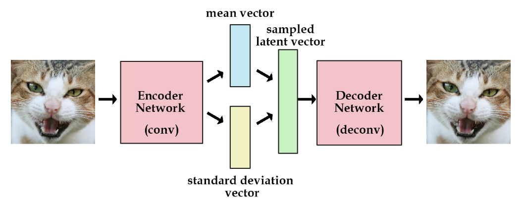
Variational AutoEncoders (VAE)
Something we cannot do with classic autoencoders is to generate data. Why is this the case?
During training time, we feed the input image and make the model learn the encoder and decoder parameters required to reconstruct the image again.
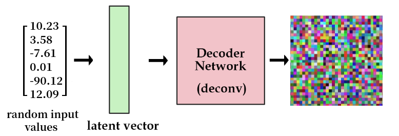
During testing time, we only need the decoder part because this is the part that generates the image. And to generate an image, we need to input some vector. However, we have no idea about the nature of this vector.
If we just give as input some random values, more likely than not, we will end up with an image that will not look like anything coherent.
So, what we do to solve this issue? We add a constraint on the encoding part of the network that forces it to generate latent vectors that roughly follow a unit gaussian distribution. By doing so, we can sample meaningful values and create a valid latent vector.
Vector Quantised-Variational AutoEncoder (VQ-VAE)
Normal VAEs learn a continuous latent representation, each value can be taken a decoded back to an image. Learning effective representation given the massive set of possibilities is hard for the model.
Instead, we want to restrict the possible number of latent vectors so the model can concentrate on these, in other words, we want a discrete latent representation.
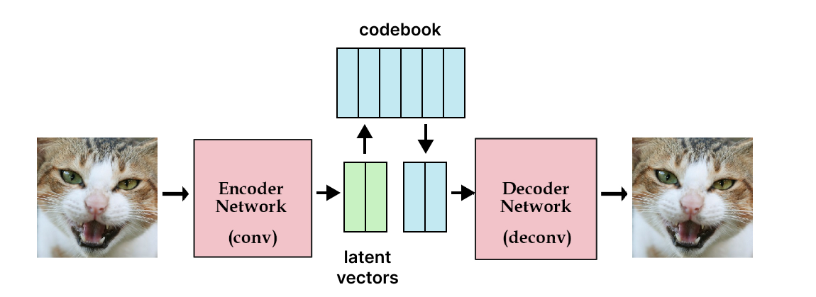
To do so, we will use vector quantization. The idea is to use a codebook, a learned collection of vectors used to create the latent vectors. In practice, we first encode an image using the encoder, obtaining multiple latent vectors.
Then, we replace all the latent by the corresponding closest vector in the codebook. We had to output more than one latent per image to have a combination of vectors taken from the codebook, it allows us to search in a bigger space but still discrete.
Applications for autoencoders in computer vision
Now that we know the types of autoencoders, lets take a look at ways they can be applied for tangible use cases. Well-known applications of autoencoders are image denoising, image inpainting, image compression and dimensionality reduction. Below we highlight other computer vision use cases in more detail.
Autoencoders in anomaly detection
Autoencoders are a very powerful tool for detecting anomalies. Through the process of encoding and decoding, you will know how well you can normally reconstruct your data. If an autoencoder is then presented with unusual data that shows something the model has never seen before, the error when reconstructing the input after the code will be much higher.
For example, a model that does a decent job at reducing and rebuilding cat images would do a very poor job when presented with, for instance, a picture of a giraffe. Reconstruction error is a very good indicator of anomalies, even for very complex and high-dimensional datasets.
Autoencoders in segmentation tasks
With autoencoders, we typically have an input image and we reconstruct the same input image by going through the autoencoder architecture. Instead of using the same input as our expected output, what if we provide a segmentation mask as the expected output? In this way, we would be able to perform tasks like semantic segmentation. Indeed, this is actually what is done by U-Net which is an autoencoder architecture usually used for semantic segmentation for biomedical images.
Applying super-resolution
Super-resolution essentially means to increase the resolution of a low-resolution image. In principle, this can also be achieved just by upsampling the image and using bilinear interpolation to fill in the new pixel values, but then the generated image will be blurry as we cannot increase the amount of information in the image. To combat this problem, we can teach an autoencoder to predict the pixel values for the high-resolution image.
Generating new data
Variational Autoencoders can be used to generate both image and time series data. The parameterized distribution at the code of the autoencoder can be randomly sampled to generate discrete values for latent vectors, which can then be forwarded to the decoder, leading to the generation of image data. Variational Autoencoders can also be used to model time series data like music.
Conclusion
Now that you have background knowledge about autoencoders, you might be interested in learning about other key topics in artificial intelligence and machine learning such as liquid neural networks or starting your first computer vision project with Roboflow. Put your new knowledge to use!
Cite this Post
Use the following entry to cite this post in your research:
Petru P.. (Oct 21, 2022). What is an Autoencoder?. Roboflow Blog: https://blog.roboflow.com/what-is-an-autoencoder-computer-vision/