
Contrast preprocessing adjusts pixel intensities on a relative basis to sharpen edges in images, which improves a computer vision model's ability to detect object boundaries during training. It is most useful when a dataset contains images with low or saturated contrast, such as scanned documents used for OCR, where distinguishing fine details from a flat background is critical. Three main techniques covered are Adaptive Equalization, Contrast Stretching, and Histogram Equalization, each suited to different contrast problems.
Adding contrast to images is a simple yet powerful technique to improve our computer vision models. But why?
When considering how to add contrast to images and why we add contrast to images in computer vision, we must start with the basics. What is contrast? How contrast preprocessing improve our models? When should we add contrast?
What Is Contrast?
Contrast, at its core, is the condition of observable difference(s). In images, this means we capture the subject's clear differences. In the most atomic terms, this means pixels vary widely from one another.
Critically, contrast does not apply a blanket filter to increased/decrease all pixels by, say, 20 percent brightness. Instead, pixels in an image are adjusted on a relative basis: darker pixels are "smoothed" across the entire image. (We'll see more on this later.)
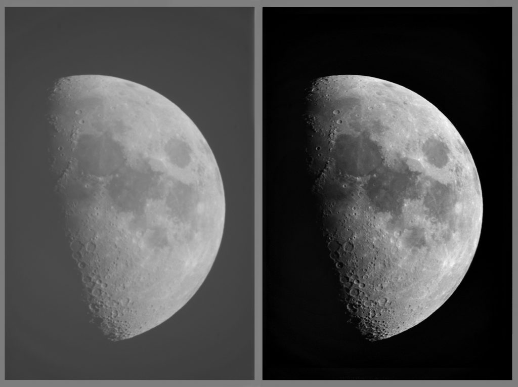
Consider two images of the same subject at the same time: the moon. Our image on the left is low contrast, while the image on the right is higher contrast.
Why Use Preprocess Images with Contrast?
In comparing our moon images, it isn't only that the image on the right looks more pleasing, it also would be easier for our neural networks to understand. Recall a fundamental tenant in computer vision (whether classification, object detection, or segmentation) is edge detection. When using contrast preprocessing, edges become clearer as neighboring pixel differences are exaggerated.
Recall the difference between preprocessing and augmentation: preprocessing images means all images in our training, validation, and test sets should undergo the transformations we apply. Augmentation only applies to our training set.
When to Use Contrast Preprocessing
In general, if a problem is believed to have images of low contrast or a portion of images with saturated contrast, smoothing the contrast of the image with preprocessing is helpful.
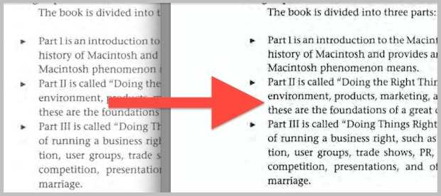
A common task where contrast is lower than desired is in processing scanned documents. In the case of low contrast, it can be challenging to deduce faint letters for optical character recognition (OCR). Creating greater contrast between the letters and the background makes clearer edges. Note that the contrast change is not simply making the entire image darker: the white background is a nearly equal shade.
How to Use Contrast Preprocessing
Contrast preprocessing can be implemented in many open source frameworks, like image contrast in TensorFlow, image contrast preprocessing in PyTorch, and adjusting image contrast in FastAI, and histogram equalization contrast in scikit-image.
Note: applying contrast within a single framework can be problematic if you later need to migrate to another framework, since implementations are not always identical.
Contrast Preprocessing in scikit-image
The scikit-image documentation contains a great representation of how image contrast affects an image's attributes.
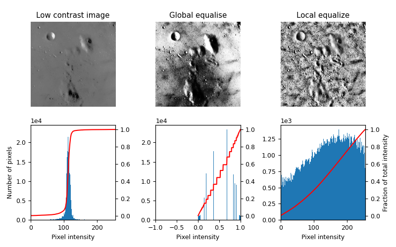
Note contrast is the act of contrast adjustment (Adaptive histogram equalization, AHE)is largely 'spreading' darker pixels more evenly across the image. This example also introduces a fundamental concept in improving contrast: local equalization.
Contrast adjustments like adaptive equalization take into account local portions of an image to prevent outcomes like the center middle image, and instead spread contrast changes more evenly across the whole image.
The script to reproduce the above output is available in the documentation:
import numpy as np
import matplotlib
import matplotlib.pyplot as plt

from skimage import data
from skimage.util.dtype import dtype_range
from skimage.util import img_as_ubyte
from skimage import exposure
from skimage.morphology import disk
from skimage.morphology import ball
from skimage.filters import rank


matplotlib.rcParams['font.size'] = 9


def plot_img_and_hist(image, axes, bins=256):
    """Plot an image along with its histogram and cumulative histogram."""
    ax_img, ax_hist = axes
    ax_cdf = ax_hist.twinx()

    # Display image
    ax_img.imshow(image, cmap=plt.cm.gray)
    ax_img.set_axis_off()

    # Display histogram
    ax_hist.hist(image.ravel(), bins=bins)
    ax_hist.ticklabel_format(axis='y', style='scientific', scilimits=(0, 0))
    ax_hist.set_xlabel('Pixel intensity')

    xmin, xmax = dtype_range[image.dtype.type]
    ax_hist.set_xlim(xmin, xmax)

    # Display cumulative distribution
    img_cdf, bins = exposure.cumulative_distribution(image, bins)
    ax_cdf.plot(bins, img_cdf, 'r')

    return ax_img, ax_hist, ax_cdf


# Load an example image
img = img_as_ubyte(data.moon())

# Global equalize
img_rescale = exposure.equalize_hist(img)

# Equalization
footprint = disk(30)
img_eq = rank.equalize(img, footprint=footprint)


# Display results
fig = plt.figure(figsize=(8, 5))
axes = np.zeros((2, 3), dtype=object)
axes[0, 0] = plt.subplot(2, 3, 1)
axes[0, 1] = plt.subplot(2, 3, 2, sharex=axes[0, 0], sharey=axes[0, 0])
axes[0, 2] = plt.subplot(2, 3, 3, sharex=axes[0, 0], sharey=axes[0, 0])
axes[1, 0] = plt.subplot(2, 3, 4)
axes[1, 1] = plt.subplot(2, 3, 5)
axes[1, 2] = plt.subplot(2, 3, 6)

ax_img, ax_hist, ax_cdf = plot_img_and_hist(img, axes[:, 0])
ax_img.set_title('Low contrast image')
ax_hist.set_ylabel('Number of pixels')

ax_img, ax_hist, ax_cdf = plot_img_and_hist(img_rescale, axes[:, 1])
ax_img.set_title('Global equalise')

ax_img, ax_hist, ax_cdf = plot_img_and_hist(img_eq, axes[:, 2])
ax_img.set_title('Local equalize')
ax_cdf.set_ylabel('Fraction of total intensity')


# prevent overlap of y-axis labels
fig.tight_layout()
plt.show()
Contrast Preprocessing in Roboflow
When preparing a dataset for training, Roboflow allows you to apply contrast preprocessing in just a few steps through its dataset versioning pipeline.
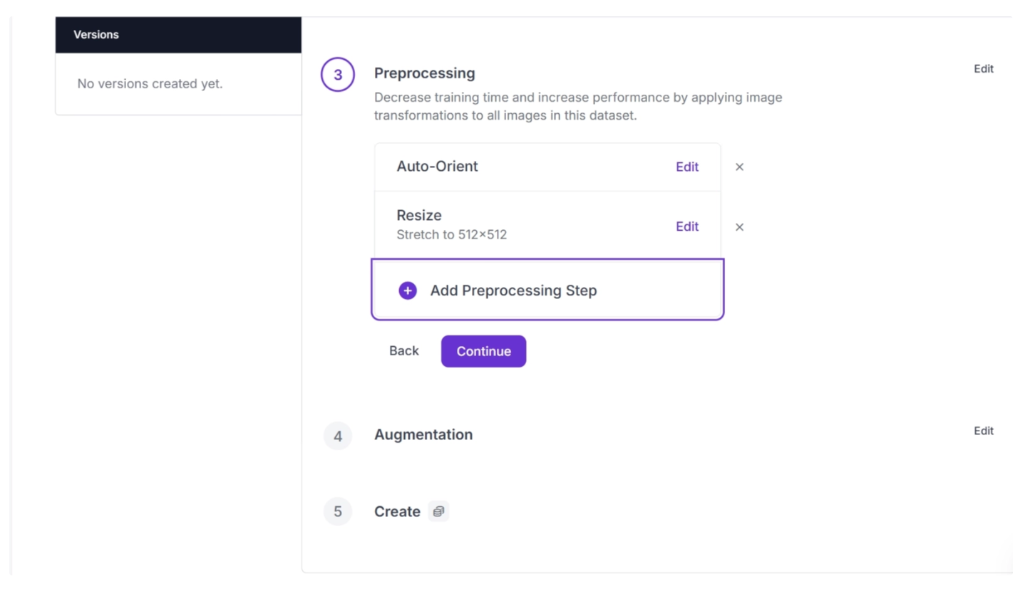
The dataset versioning pipeline in Roboflow, as shown below, is no-code and offers a complete process for preparing datasets for training models through a simple interface.
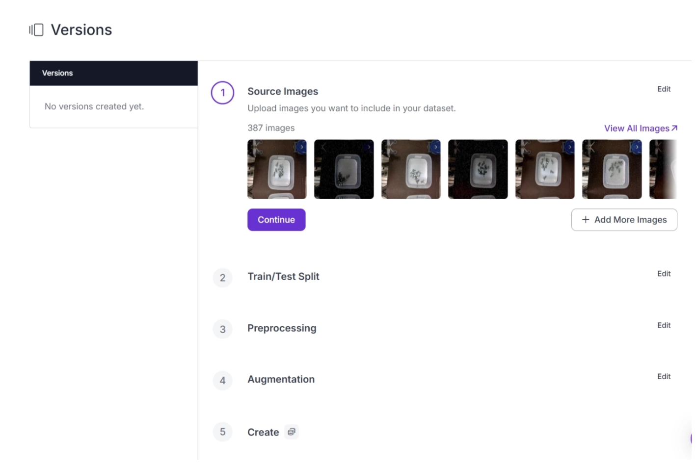
To apply contrast to all images in your dataset, add a preprocessing step as shown below.
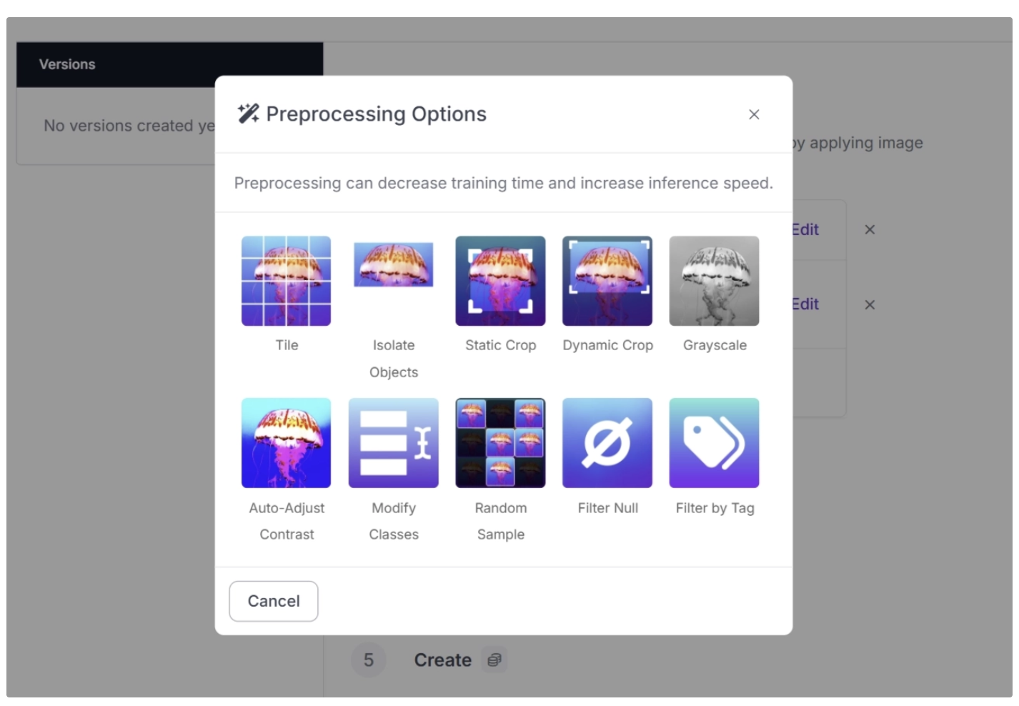
From there, you can choose from several preprocessing options. Select Auto-Adjust Contrast to apply contrast to your images.
Roboflow also offers multiple contrast techniques, each with a distinct purpose:
- Adaptive Equalization: Enhances contrast locally by adjusting small regions of the image independently, making details in both dark and bright areas more visible.
- Contrast Stretching: Expands the range of pixel intensity values so that the darkest pixels become darker and the brightest become brighter, improving overall image contrast.
- Histogram Equalization: Redistributes pixel intensities across the entire image to create a more uniform histogram, enhancing global contrast especially in low-contrast images.
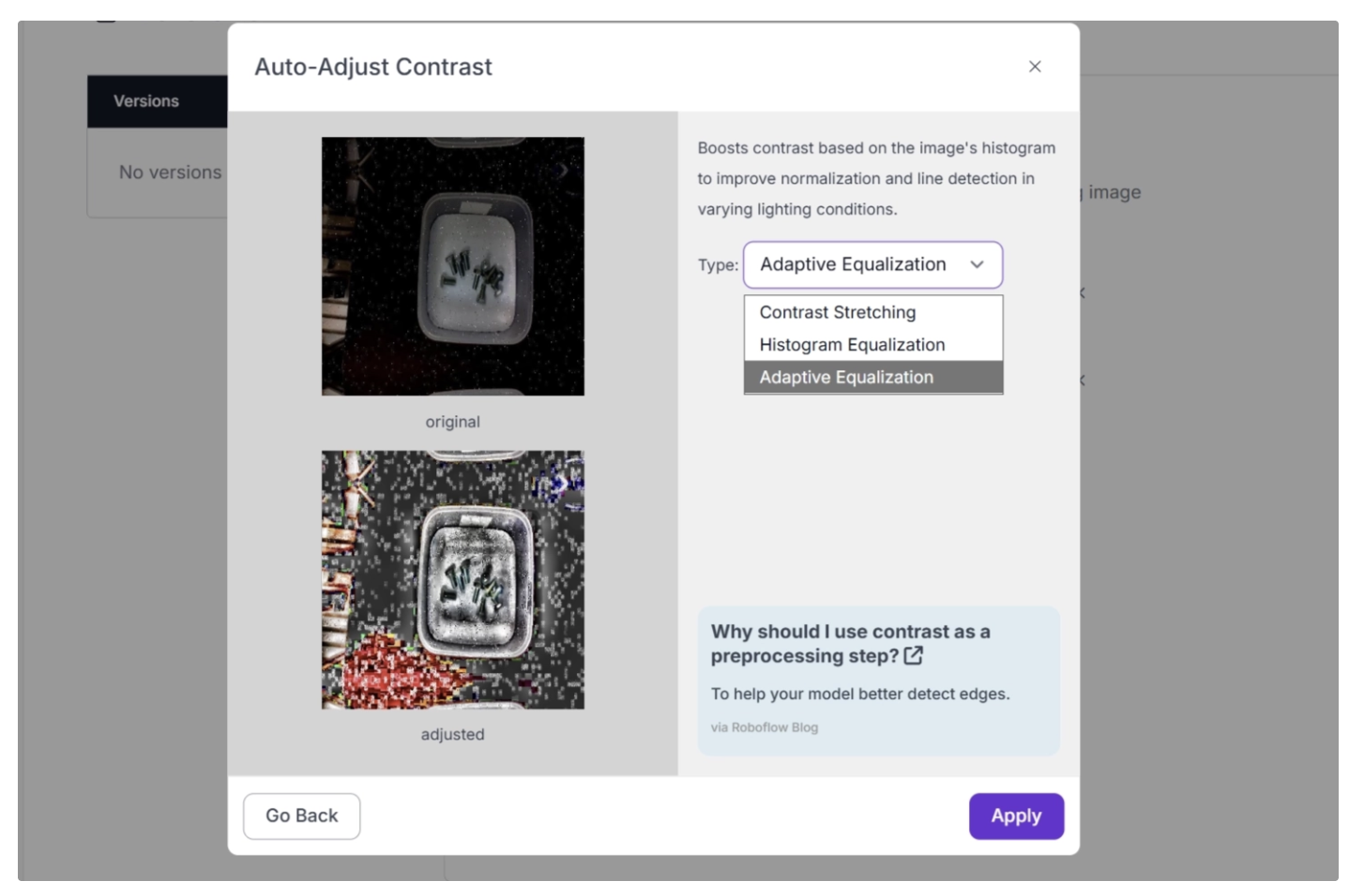
Once selected, simply apply contrast to your dataset. Additionally, the dataset versioning pipeline allows you to track, manage, and reproduce different dataset versions with preprocessing steps such as contrast.
Another advantage to Roboflow is your preprocessing is constant across your dataset, including across model frameworks. This easier empower experimentation and sampling results.
We can't wait to see what you build.
When should I use contrast preprocessing?
Use contrast preprocessing when your dataset contains images with low or saturated contrast, as it helps smooth pixel intensities to make subjects stand out. It is particularly useful for tasks like Optical Character Recognition, where defining clear edges between a faint subject and its background is critical for the model's accuracy.
Cite this Post
Use the following entry to cite this post in your research:
Dikshant Shah. (Jan 15, 2026). When to Use Contrast as a Preprocessing Step. Roboflow Blog: https://blog.roboflow.com/when-to-use-contrast-as-a-preprocessing-step/