Using YOLO-World With Active Learning to Train a Custom Model

Large vision models like YOLO-World, a zero-shot open-vocabulary object detection model by Tencent’s AI Lab, have shown impressive performance. While zero-shot detection models can detect objects with increasing accuracy, smaller custom models have proven to be faster and more compute-efficient than large models while being more accurate in specific domains and use cases.

Despite those tradeoffs, there’s an important benefit to large, zero-shot models: they require no data labeling or model training to use in production. 

In this guide, we demonstrate an approach to applying the benefits of YOLO-World while using active learning for data collection to train a custom model. To do this, we will:

1. Deploy YOLO-World using Inference
2. Integrate active learning with our deployment
3. Train a custom model using our automatically labeled data

Step 1: Deploy YOLO-World

In a few steps, we can set up YOLO-World to run on Roboflow Inference. First, we will install our required packages:

pip install -q inference-gpu[yolo-world]==0.9.12rc1

Then, we will import YOLO-World from Roboflow Inference, where we will set up the classes that we want to detect:

from inference.models.yolo_world.yolo_world import YOLOWorld

model = YOLOWorld(model_id="yolo_world/l") # There are multiple different sizes: s, m and l.

classes = ["book"] # Change this to whatever you want to detect
model.set_classes(classes)

Next, we can run an inference on a sample image and see the model in action:

import supervision as sv
import cv2

image = cv2.imread(IMAGE_PATH)
results = model.infer(image, confidence=0.2) # Infer several times and play around with this confidence threshold
detections = sv.Detections.from_inference(results)

Using Supervision, we can visualize the predictions:

labels = [
    f"{classes[class_id]} {confidence:0.3f}"
    for class_id, confidence
    in zip(detections.class_id, detections.confidence)
]


annotated_image = image.copy()
annotated_image = sv.BoundingBoxAnnotator().annotate(annotated_image, detections)
annotated_image = sv.LabelAnnotator().annotate(annotated_image, detections, labels=labels)
sv.plot_image(annotated_image)

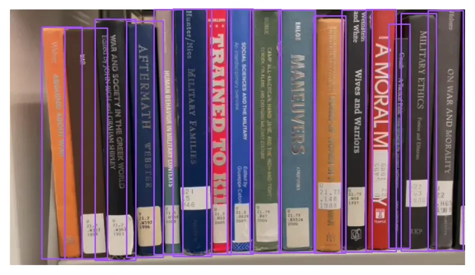
Now we can start running predictions with YOLO-World, and with a bit of extra code, we can start to create a model that’s faster, more efficient, and more accurate at the same time.

Step 2: Active Learning

First, to have a place to store our data, we will create a Roboflow project for our book detection model. 

Once that’s done, we can access our workspace with the Roboflow API using Python. First, let’s install the Roboflow Python SDK:

pip install roboflow

Then, we can access our project by using our API key and entering our workspace and project ID.   

from roboflow import Roboflow

rf = Roboflow(api_key="YOUR_ROBOFLOW_API_KEY")
project = rf.workspace("*workspace_id*").project("*project_id*")

After that, we have all we need to combine all the previous parts of this guide to create a function that we can use to predict with YOLO-World, while adding those predictions to a dataset so we can train a custom model.

from inference.models.yolo_world.yolo_world import YOLOWorld
import supervision as sv
import cv2
from roboflow import Roboflow


# Project Setup (Copied From Previous Section)
rf = Roboflow(api_key="YOUR_ROBOFLOW_API_KEY")
project = rf.workspace("*workspace_id*").project("*project_id*")


# Model Setup (Copied From Previous Section)
model = YOLOWorld(model_id="yolo_world/l") # There are multiple different sizes: s, m and l.
classes = ["book"] # Change this to whatever you want to detect
model.set_classes(classes)


def infer(image):
 results = model.infer(image, confidence=0.1)
 detections = sv.Detections.from_inference(results)

 image_id = str(uuid.uuid4())
 image_path = image_id+".jpg"
 dataset = sv.DetectionDataset(classes=classes,images={image_path:image},annotations={image_path:detections})
 dataset.as_pascal_voc("dataset_upload/images","dataset_upload/annotations")
  project.upload(
     image_path=f"dataset_upload/images/{image_path}",
     annotation_path=f"dataset_upload/annotations/{image_id}.xml",
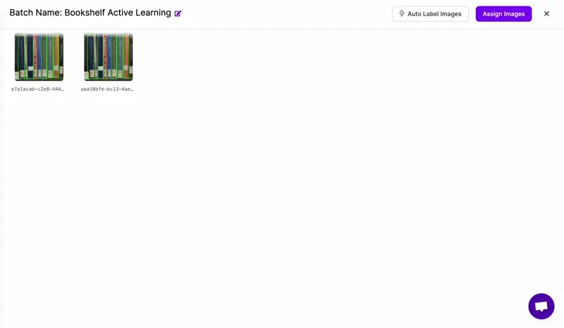
     batch_name="Bookshelf Active Learning",
     is_prediction=True
 )

 return detections

You can change the infer function to suit your deployment needs. For our example, we plan to run detections on a video, and we don’t want nor need every single frame to be uploaded, so we will modify our infer function to upload randomly 25% of the time:

def infer(image):
  results = model.infer(image, confidence=0.1)
  detections = sv.Detections.from_inference(results)

  if random.random() < 0.25:
    print("Adding image to dataset")

    image_id = str(uuid.uuid4())
    image_path = image_id+".jpg"
    dataset = sv.DetectionDataset(classes=classes,images={image_path:image},annotations={image_path:detections})
    dataset.as_pascal_voc("dataset_upload/images","dataset_upload/annotations")
    
    project.upload(
        image_path=f"dataset_upload/images/{image_path}",
        annotation_path=f"dataset_upload/annotations/{image_id}.xml",
        batch_name="Bookshelf Active Learning",
        is_prediction=True
    )

  return detections

Using Supervision and the following code, we will run inferences against a video of a library:

def process_frame(frame, i):
  print(i)
  detections = infer(frame)

  annotated_image = frame.copy()
  annotated_image = sv.BoundingBoxAnnotator().annotate(annotated_image, detections)

  return annotated_image

sv.process_video("library480.mov","library_processed.mp4",process_frame)

Then, as you run inferences, you will see images being added to your Roboflow project.

Once uploaded, you can review and correct annotations as necessary, then create a new version to start training your custom model!

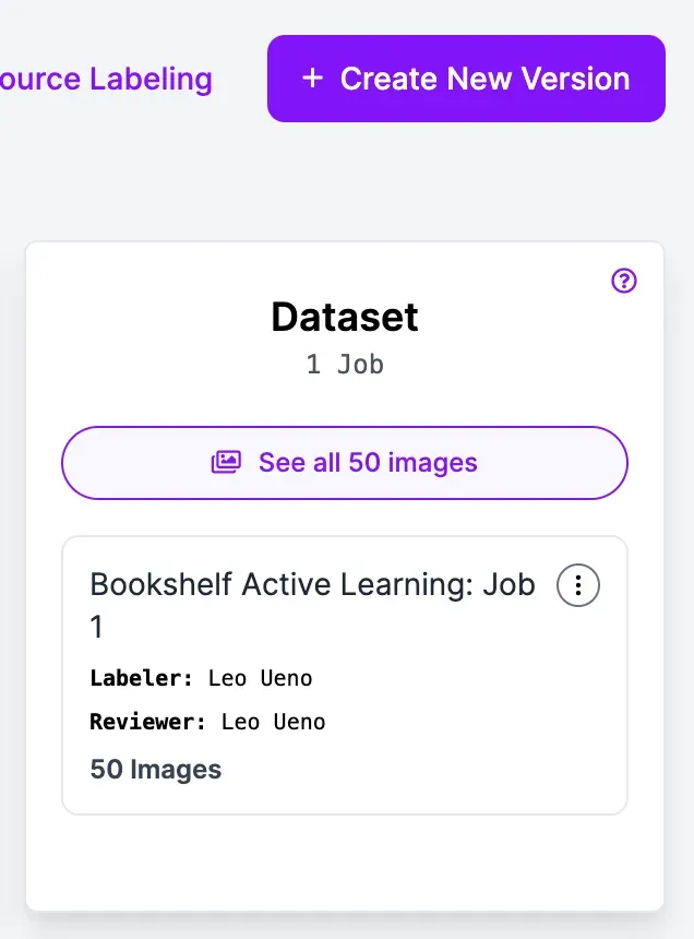
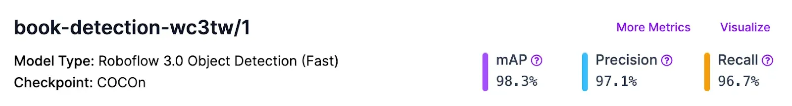
After training, we were able to train a custom model with around 98.3% mean average precision (mAP).

As you continue using your model, whether that be a custom model or a large model like YOLO-World, you can continue collecting data to further improve our models in the future.

Conclusion

In this guide, we were able to combine the best of both worlds: Using a state-of-the-art zero-shot object detection model for immediate use and then using that deployed model to train a custom model with better performance without spending time collecting and labeling a dataset.

After you create your custom model, you can keep improving your models through built-in active learning features in the Roboflow platform.