
Have you ever wondered how you can estimate the speed of vehicles using computer vision? In this tutorial, I'll explore the entire process, from object detection to tracking to speed estimation.
Along the way, I confronted the challenges of perspective distortion and learned how to overcome them with a bit of math!
This blog post contains short code snippets. Follow along using the open-source notebook we have prepared, where you will find a full working example. We have also released several scripts compatible with the most popular object detection models, which you can find here.
Object Detection for Speed Estimation
Let's start with detection. To perform object detection on the video, we need to iterate over the frames of our video, and then run our detection model on each of them. The Supervision library handles video processing and annotation, while Inference provides access to pre-trained object detection models. We specifically load the rf-detr-base-640 model from Roboflow.
If you want to learn more about object detection with the Inference, visit the Inference GitHub repository and documentation.
import supervision as sv
from inference.models.utils import get_roboflow_model

model = get_roboflow_model('rf-detr-base-640')
frame_generator = sv.get_video_frames_generator('vehicles.mp4')
bounding_box_annotator = sv.BoundingBoxAnnotator()

for frame in frame_generator:
    results = model.infer(frame)[0]
    detections = sv.Detections.from_inference(results)

    annotated_frame = trace_annotator.annotate(
scene=frame.copy(), detections=detections)Detecting vehicles with Inference
In our example we used Inference, but you can swap it for RF-DETR or any other model. You need to change a few lines in your code, and you should be good to go.
import supervision as sv
from inference.models.utils import get_roboflow_model

model = get_roboflow_model('rf-detr-base-640')
frame_generator = sv.get_video_frames_generator('vehicles.mp4')
bounding_box_annotator = sv.BoundingBoxAnnotator()

for frame in frame_generator:
    results = model.infer(frame)[0]
    detections = sv.Detections.from_inference(results)

    annotated_frame = trace_annotator.annotate(
        scene=frame.copy(), detections=detections)
Multi-Object Tracking for Speed Estimation
Object detection is not enough to perform speed estimation. To calculate the distance traveled by each car we need to be able to track them. For this, we use BYTETrack, accessible in the Supervision pip package.
...

# initialize tracker
byte_track = sv.ByteTrack()

...

for frame in frame_generator:
    results = model.infer(frame)[0]
    detections = sv.Detections.from_inference(results)

    # plug the tracker into an existing detection pipeline
    detections = byte_track.update_with_detections(detections=detections)

    ...
If you want to learn more about integrating BYTETrack into your object detection project, head over to the Supervision docs page. There, you will find an end-to-end example showing how you can do it with different detection models.
Tracking vehicles using BYTETrack
Perspective Distortion in Distance Measurement
Let's consider a simplistic approach where the distance is estimated based on the number of pixels the bounding box moves.
Here's what happens when you use dots to memorize the position of each car every second. Even when the car moves at a consistent speed, the pixel distance it covers varies. The further away it is from the camera, the smaller the distance it covers.
Impact of perspective distortion on the number of covered pixels
As a result, it will be very hard for us to use raw image coordinates to calculate the speed. We need a way to transform the coordinates in the image into actual coordinates on the road, removing the perspective-related distortion along the way. Fortunately, we can do this with OpenCV and some mathematics.
Math Behind Perspective Transformation
To transform the perspective, we need a Transformation Matrix, which we determine using the getPerspectiveTransform function in OpenCV. This function takes two arguments - source and target regions of interest. In the visualization below, these regions are labeled A-B-C-D and A'-B'-C'-D', respectively.
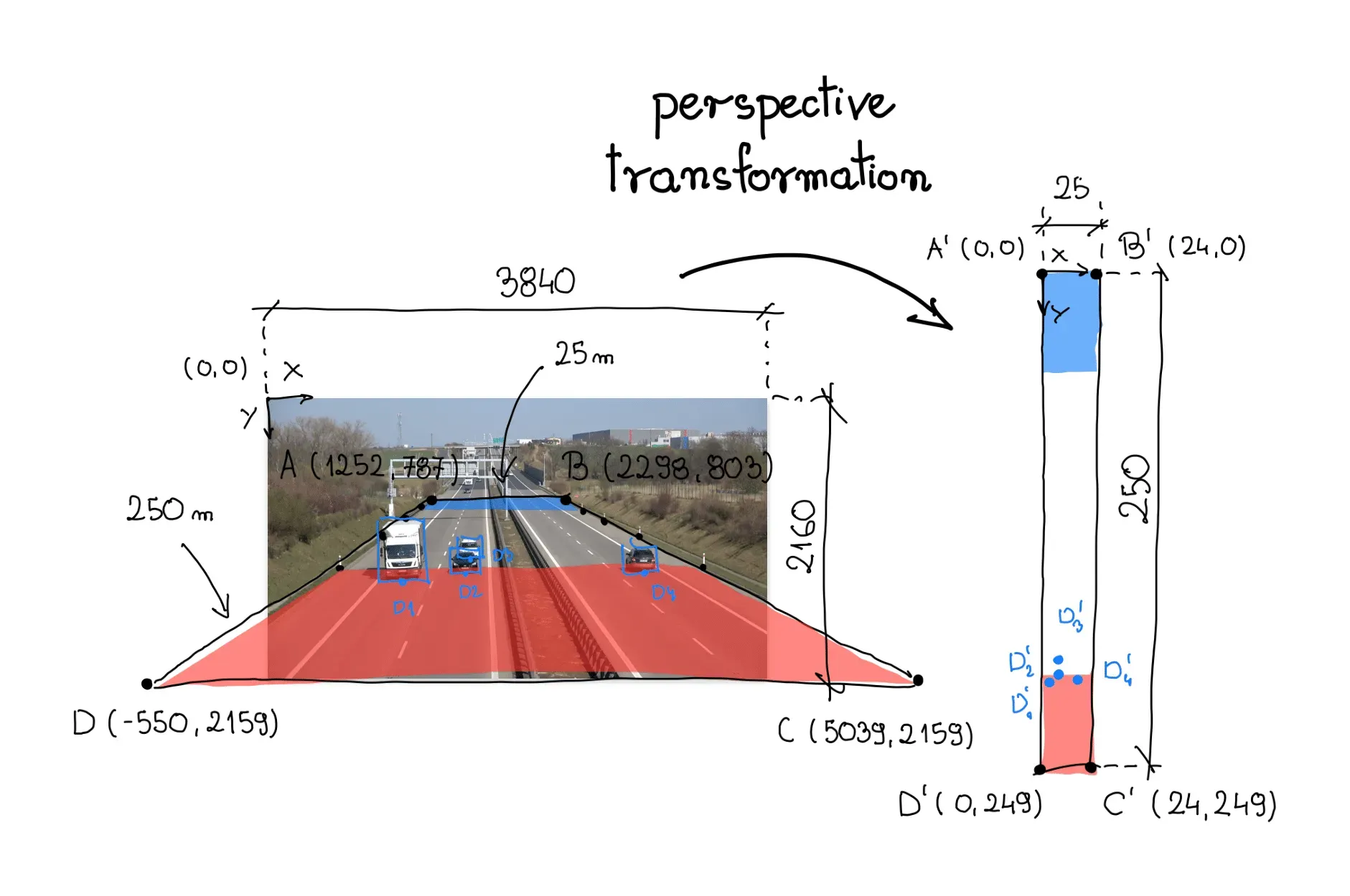
Analyzing a single video frame, I chose a stretch of road that would serve as the source region of interest. On the shoulders of highways, there are often vertical posts - markers, spaced every fixed distance. In this case, 50 meters. The region of interest spans the entire width of the road and the section connecting the six aforementioned posts.
In our case, we are dealing with an expressway. Research in Google Maps showed that the area surrounded by the source region of interest measures approximately 25 meters wide and 250 meters long. We use this information to define the vertices of the corresponding quadrilateral, anchoring our new coordinate system in the upper left corner.
Finally, we reorganize the coordinates of vertices A-B-C-D and A'-B'-C'-D' into 2D SOURCE and TARGET matrices, respectively, where each row of the matrix contains the coordinates of one point.
SOURCE = np.array([
    [1252, 787],
    [2298, 803],
    [5039, 2159],
    [-550, 2159]
])

TARGET = np.array([
    [0, 0],
    [24, 0],
    [24, 249],
    [0, 249],
])
Perspective Transformation
Using the source and target matrices, we create a ViewTransformer class. This class uses OpenCV's getPerspectiveTransform function to compute the transformation matrix. The transform_points method applies this matrix to convert the image coordinates into real-world coordinates.
class ViewTransformer:
    def __init__(self, source: np.ndarray, target: np.ndarray) -> None:
        source = source.astype(np.float32)
        target = target.astype(np.float32)
        self.m = cv2.getPerspectiveTransform(source, target)

    def transform_points(self, points: np.ndarray) -> np.ndarray:
        if points.size == 0:
            return points

        reshaped_points = points.reshape(-1, 1, 2).astype(np.float32)
        transformed_points = cv2.perspectiveTransform(
                reshaped_points, self.m)
        return transformed_points.reshape(-1, 2)

view_transformer = ViewTransformer(source=SOURCE, target=TARGET)
Logic responsible for perspective transformation
Object coordinates after perspective transformation
Calculating Speed with Computer Vision
We now have our detector, tracker, and perspective conversion logic in place. It's time for speed calculation. In principle, it's simple: divide the distance covered by the time it took to cover that distance. However, this task has its complexities.
In one scenario, we could calculate our speed every frame: calculate the distance traveled between two video frames and divide it by the inverse of our FPS, in my case, 1/25. Unfortunately, this method can result in very unstable and unrealistic speed values.
To prevent this, we average the values obtained throughout one second. This way, the distance covered by the car is significantly larger than the small box movement caused by flickering, and our speed measurements are closer to the truth.
...

video_info = sv.VideoInfo.from_video_path('vehicles.mp4')

# initialize the dictionary that we will use to store the coordinates
coordinates = defaultdict(lambda: deque(maxlen=video_info.fps))

for frame in frame_generator:
    results = model.infer(frame)[0]
    detections = sv.Detections.from_inference(results)
    detections = byte_track.update_with_detections(detections=detections)

    points = detections.get_anchors_coordinates(
        anchor=sv.Position.BOTTOM_CENTER)

    # plug the view transformer into an existing detection pipeline
    points = view_transformer.transform_points(points=points).astype(int)

    # store the transformed coordinates
    for tracker_id, [_, y] in zip(detections.tracker_id, points):
        coordinates[tracker_id].append(y)

    for tracker_id in detections.tracker_id:

        # wait to have enough data
        if len(coordinates[tracker_id]) > video_info.fps / 2:

            # calculate the speed
            coordinate_start = coordinates[tracker_id][-1]
            coordinate_end = coordinates[tracker_id][0]
            distance = abs(coordinate_start - coordinate_end)
            time = len(coordinates[tracker_id]) / video_info.fps
            speed = distance / time * 3.6
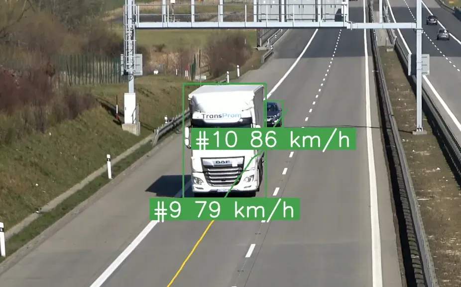
...Result speed estimation visualization
Hidden Complexities with Speed Estimation
Many additional factors should be considered when building a real-world vehicle speed estimation system. Let's briefly discuss a few of them.
Occluded and trimmed boxes: The stability of the box is a key factor affecting the quality of speed estimation. Small changes in the size of the box when one car temporarily obscures another can lead to large changes in the value of the estimated speed.
Setting a fixed reference point: In this example, we used the bottom center of the bounding box as a reference point. This is possible because the weather conditions in the video are good - a sunny day, no rain. However, it is easy to imagine situations where locating this point can be much more difficult.
The slope of the road: In this example, it is assumed that the road is completely flat. In reality, this rarely happens. To minimize the impact of the slope, we must limit ourselves to the part where the road is relatively flat, or include the slope in the calculations.
Conclusion
There is so much more you can do with speed estimation. For example, the below video shows color-codes cars based on car speed. I hope this blog post will inspire you to build something even cooler.
An example application that marks cars with different colors based on their estimated speed
Stay up to date with the projects we are working on at Roboflow and on my GitHub! Most importantly, let us know what you've been able to build.
Cite this Post
Use the following entry to cite this post in your research:
Piotr Skalski. (Jan 19, 2024). How to Estimate Speed with Computer Vision. Roboflow Blog: https://blog.roboflow.com/estimate-speed-computer-vision/