
We're often told that data is the backbone that drives the development of powerful and robust models. And that's certainly true – data is the raw material that we feed into our algorithms, helping them to learn, adapt, and make predictions. However, not just any data will suffice.
High-quality, clean data is what truly makes the difference when it comes to training computer vision models. "Garbage in, garbage out" is an adage as old as data processing itself, and it reminds us that the quality of our input data is just as crucial, if not more so.
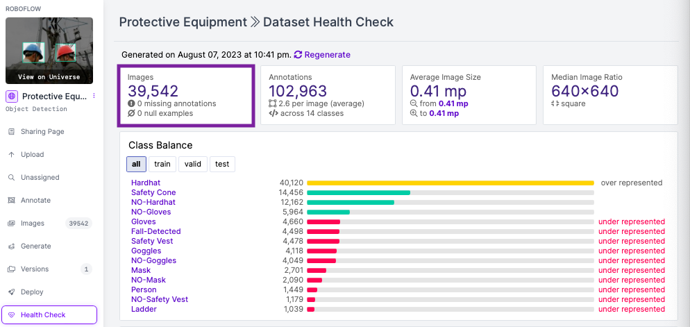
In this experiment, we sought to explore whether downsizing the dataset without losing significant accuracy was achievable. By carefully pruning over 10k images that were either outliers, blurry, or duplicates, we managed to reduce the dataset size by nearly 26% while maintaining a mAP score of 76.5% with RF-DETR, compared to 79% on the original dataset.
So, is this 3% drop in mAP worth it? Let's consider some factors:
- Efficiency: Reducing the dataset size by such a significant margin could lead to more efficient training and lower computational costs. This could be particularly valuable in scenarios where resources are constrained.
- Quality Control: By eliminating ambiguous or poor-quality images, the dataset may become more consistent, leading to a model that performs more robustly in specific real-world scenarios.
- Practical Impact: A 3% drop in mAP might be acceptable depending on the application. If the model is being used in a context where absolute top performance is not critical, the trade-off might be quite favorable.
- Potential Overfitting: Reducing the presence of noisy or irrelevant data might even help in preventing overfitting, allowing the model to generalize better to unseen data.
However, it's essential to consider the specific requirements of the task at hand:
- If the application demands the highest possible accuracy and every percentage point is vital, this reduction might not be suitable.
- If there are other factors such as the need for faster prototyping, lower costs, or a focus on higher-quality data, this 3% trade-off could indeed be considered a success.
The value of this approach depends on a complex interplay of factors including efficiency, application requirements, and the quality of the data itself. In our case, the slight decrease in mAP seems to be a reasonable trade-off for a more refined and efficient dataset. However, as with many aspects of machine learning, the 'right' approach depends on the specific context and goals of the project.
Introduction
In this blog post, we'll be exploring an intricate yet practical approach to data management for efficient model training. We'll demonstrate how to achieve the same model accuracy with less data by cleaning our dataset effectively. We'll use a comprehensive example using a personal protective equipment dataset of over 39,000 images and the RF-DETR object detection model, showcasing the use of libraries such as roboflow, ultralytics and fastdup.
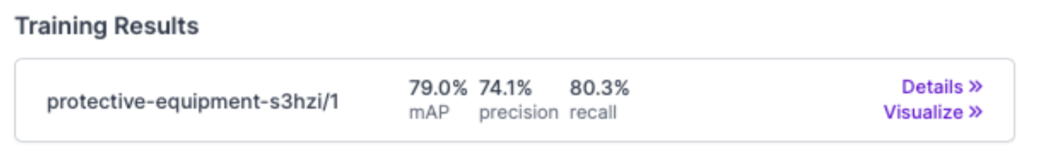
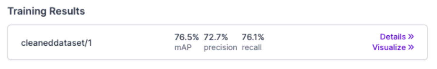
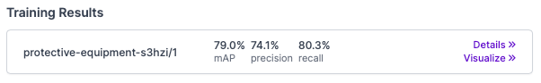
Comparison of training results: Left, the original dataset achieving a mean average precision (mAP) of 0.79; Right, the cleaned dataset yielding a slightly lower mAP of 0.76. Illustrating the effective downsizing of data without a significant loss in accuracy.
By the end of this post, we will prune over 10,500 images that are blurry, duplicates, and outlier images reducing our dataset by a significant amount. With a smaller clean dataset, you can reduce labeling costs and computation costs while maintaining the accuracy of your model.
Identifying and Addressing Suboptimal Data
To optimize a dataset, we should identify and address suboptimal data. This includes:
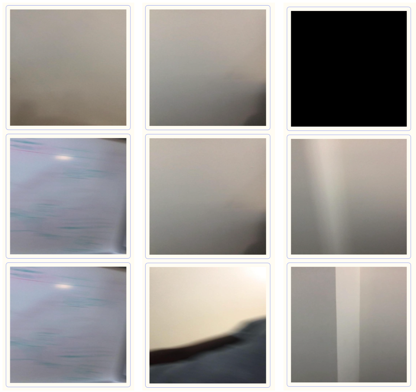
- Duplicates or highly similar images: These could lead to overfitting and bias. Removing them ensures dataset diversity.
- Outlier images: These are images that are significantly different from the majority of images in our dataset. They could vary in terms of color distribution, object orientation, or presence of unusual elements. Outliers may distract the model during the training phase and lower its performance.
- Blurry images: Low-quality images reduce accuracy as they don't provide clear features.
- Dark or bright images: Extreme lighting conditions hinder feature identification and learning.
With this understanding, we can now outline the steps we'll follow in this guide:
- Install Libraries
- Download Dataset
- Train on Original Data
- Analyzing the Dataset with Fastdup
- Identify invalid, duplicate, and outlier images
- Remove duplicates, outliers, and blurry images
- Train and Re-deploy
Step 1: Install Libraries
We will utilize roboflow for managing and downloading dataset, fastdup for analyzing and cleaning the dataset, and RF-DETR for training the model.
!pip -q install roboflow fastdup ultralyticsStep 2: Downloading the Dataset
Roboflow is a comprehensive tool for managing computer vision workflows. It offers a suite of features, including data labeling, versioning, and a library of public datasets known as "Roboflow Universe". This tool simplifies data acquisition and management for your projects.
To download a dataset, use the following code:
roboflow.login()
rf = Roboflow()
project = rf.workspace("roboflow-ngkro").project("protective-equipment-s3hzi")
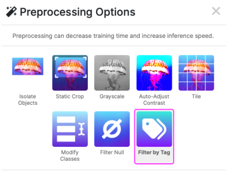
dataset = project.version(1).download("yolov8")You can further refine your datasets using Roboflow's features like the "Filter by Tag" preprocessing tool.
Step 3: Train on Original Data
Before we clean the dataset, we can train the model on the original dataset to benchmark its performance. This is optional but could provide insightful context. We use the RF-DETR model for training with pre-trained weights for 100 epochs and reached 0.79 on mAP50. You can try the deployed pre-trained model here.
model = YOLO('yolov8n.pt')
model.train(data=dataset.location + '/data.yaml', epochs=100, imgsz=640)
Step 4: Analyzing the Dataset with Fastdup
To ensure that our model is not overfitting due to duplicate or very similar images, we use the Fastdup library to analyze our dataset. We analyze the training, testing, and validation datasets separately.
fd_train = fastdup.create(work_dir="./train/", input_dir=dataset.location + '/train/images')
fd_train.run()
fd_test = fastdup.create(work_dir="./test/", input_dir=dataset.location + '/test/images')
fd_test.run()
fd_valid = fastdup.create(work_dir="./valid/", input_dir=dataset.location + '/valid/images')
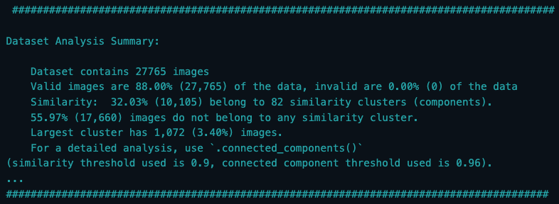
fd_valid.run()This will output a detailed analysis summary as shown below, providing information about the similarities within your dataset. You'll learn the total number of images, how many of those are considered valid, the percentage of similarity, the number and percentage of outliers, and more.
Step 5: Identify Invalid, Duplicate, and Outlier Images
Duplicate Images
FastDup allows us to visually inspect duplicate or near-duplicate images in our dataset. By identifying and removing these, we can reduce the size of our dataset without negatively affecting the diversity of our data.
We create reports for each dataset using:
fd_train.vis.duplicates_gallery()
fd_test.vis.duplicates_gallery()
fd_valid.vis.duplicates_gallery()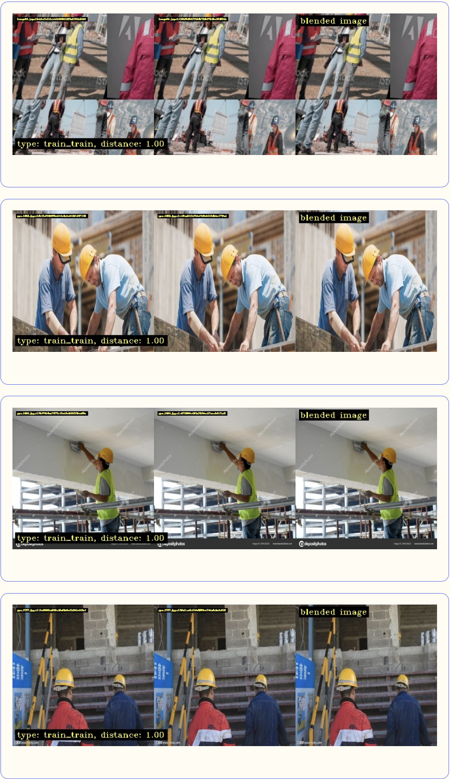
Using the reports, we can visualize the duplicate images. We first find the connected components in our image dataset. The connected_components() function returns a DataFrame with information about the connected components in the dataset and we group the connected components. These components represent clusters of similar images in our dataset. Then, we process clusters for each set.
cluster_images_to_keep_train, list_of_duplicates_train = process_clusters(clusters_df_train)
cluster_images_to_keep_test, list_of_duplicates_test = process_clusters(clusters_df_test)
cluster_images_to_keep_valid, list_of_duplicates_valid = process_clusters(clusters_df_valid)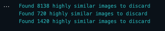
Outlier Images
Then, we can identify outlier images. Outliers are images that are dissimilar to the majority of images in our dataset. However, this doesn't necessarily mean that these images are problematic or irrelevant; they could just be distinct in some aspects (such as color distribution, texture, object presence, etc.), leading to their high-distance classification. Using a specific threshold, we can identify these outliers and remove them from our dataset after verifying, ensuring our model is not distracted by these instances.
outlier_df_train = fd_train.outliers()
list_of_outliers_train = outlier_df_train[outlier_df_train.distance < 0.68].filename_outlier.tolist()
outlier_df_test = fd_test.outliers()
list_of_outliers_test = outlier_df_test[outlier_df_test.distance < 0.68].filename_outlier.tolist()
outlier_df_valid = fd_valid.outliers()
list_of_outliers_valid = outlier_df_valid[outlier_df_valid.distance < 0.68].filename_outlier.tolist()
Dark, Bright, and Blurry Images
Step 6: Remove Duplicates, Outliers, and Blurry Images
After visualizing the reports and verifying the images, we can save the duplicate, blurry, dark, bright or outlier images to a list to prepare for removal. We will use delete_images function to remove the list of images we discovered. In this instance, I only remove the outlier, blurry and duplicate images.
def delete_images(list, dir_path):
num_deleted = 0
for file_path in list:
try:
os.remove(file_path)
num_deleted += 1
except Exception as e:
print(f"Error occurred when deleting file {file_path}: {e}")
print(f"Deleted {num_deleted} images")
# Count the number of images left
remaining_images = len(os.listdir(dir_path))
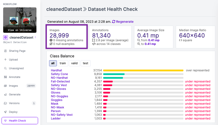
print(f"There are {remaining_images} images left in the directory {dir_path}.")With this approach, we reduced our dataset by ~26% from 39,542 to 28,999 images, maintaining a consistent model performance (mAP50) of 0.79 to XX. This technique is a practical method to conserve computational resources and time while preserving the diversity of our data and not significantly impacting model performance.
By cleaning your dataset in advance of labeling, you can significantly reduce cost and time during the labeling process.
Step 7: Train and Re-deploy
Once you have thoroughly cleaned and optimized your dataset, you can upload it back to Roboflow. This ensures streamlined integration of your refined data. After successful uploading, you can seamlessly commence the training process to attain the best possible model performance.
You can use your cleaned dataset directly using the code snippet and train using RF-DETR.
project = rf.workspace("roboflow-ngkro").project("cleaneddataset")
dataset = project.version(1).download("yolov8")
model = YOLO('yolov8n.pt')
model.train(data=dataset.location + '/data.yaml', epochs=100, imgsz=640)After cleaning the dataset, we retrained the model and observed the following:
Original dataset mAP: 0.79
Cleaned dataset mAP: 0.765

The results show that the cleaned data led to similar performance with ~26% less data while saving us a significant training time and computation cost. This emphasizes the importance of quality data management.
Deploy Your Model
After achieving a performant model on the cleaned dataset, the deployment phase is a crucial step. This is where the trained model is transitioned from a theoretical construct to a practical solution, ready to be tested.
Moving forward, you can deploy models with precision across various cloud and edge environments.
path_to_trained_weight = "./runs/detect/train"
project.version(1).deploy("yolov8", path_to_trained_weight)
Conclusion
In this tutorial, we demonstrated how to optimize a computer vision model by cleaning the dataset and removing duplicate, highly similar, or outlier images. By applying these methods, we are able to maintain the diversity of our data while reducing its size, ultimately saving computational resources and time without significantly sacrificing model performance.
Cite this Post
Use the following entry to cite this post in your research:
Arty Ariuntuya. (Aug 9, 2023). How to Reduce Dataset Size Without Losing Accuracy. Roboflow Blog: https://blog.roboflow.com/how-to-reduce-dataset-size-computer-vision/