How to Train a VGG-16 Image Classification Model on Your Own Dataset

The VGG16 model is a deep convolutional network that helped set the template for modern image classification, and it is still a reasonable choice when top accuracy matters more than speed. This guide explains what the VGG-16 model is and how it works, then shows how to train an image classification model on your own data in Roboflow, in the browser.

We use a simple flower classifier (daisy versus dandelion) as the worked example, since telling two visually similar classes apart is a clean stand-in for any single-label classification task, from sorting product photos to flagging damaged parts. The steps are the same for any set of classes, so you can swap in your own images at any point.

Explore top image classification models ranked on Roboflow Playground.

What Is the VGG-16 Model?

VGG-16 is a convolutional neural network introduced in the 2014 paper Very Deep Convolutional Networks for Large-Scale Image Recognition from the University of Oxford's Visual Geometry Group, which is where the VGG name comes from. It reaches 92.7 percent top-5 accuracy on ImageNet, which kept it a popular choice for tasks that prioritize classification accuracy.

How the VGG-16 Architecture Works

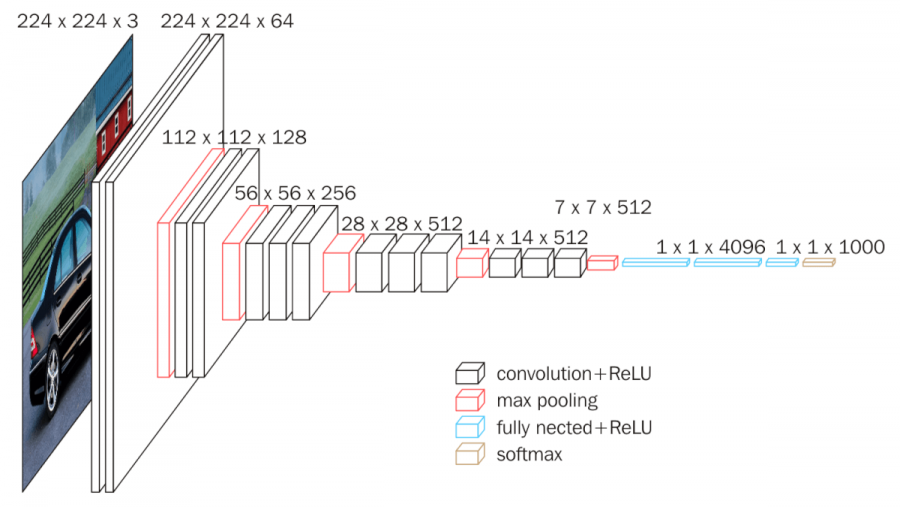
The VGG16 model is 16 weight layers deep: 13 convolutional layers followed by 3 fully connected layers. Its key design choice is using many small 3x3 convolutional filters stacked in sequence rather than a few large ones. Stacking small filters gives the network the same effective receptive field as larger filters while using fewer parameters per layer and adding more non-linearity, which lets it learn finer detail. The network takes a fixed 224x224 RGB image and passes it through blocks of convolutions and max-pooling that progressively shrink the spatial size and grow the channel depth, ending in a classifier that outputs a probability for each class.

Where the VGG-16 Model Fits Today

VGG-16 is a clear, well-documented reference for how deep classifiers are built, and its accuracy still holds up. The tradeoff is size and speed: at roughly 138 million parameters it is heavy to store and slow to run compared with newer architectures.

For classification today, Vision Transformers and residual networks like ResNet reach higher accuracy at similar or lower cost, MobileNet is the common pick for real-time and on-device use, and CLIP enables zero-shot classification from text prompts with no training at all.

You do not need to hand-configure any of these in a framework to get a working classifier. Roboflow trains an image classification model for you from an ImageNet-pretrained checkpoint, so you get the transfer-learning benefit VGG-16 popularized without managing the training code yourself.

Training an Image Classification Model

Image classification assigns one label (or a set of labels) to a whole image, answering what is this a picture of. That is different from object detection, which draws a box around each object and is the right tool when you need to locate or count things. If your question is which category does this image belong to, classification is the task, and the flower example below shows the full flow.

What you need

A free Roboflow account, a set of images sorted by the classes you care about, and a browser.

Step 1: Create a classification project

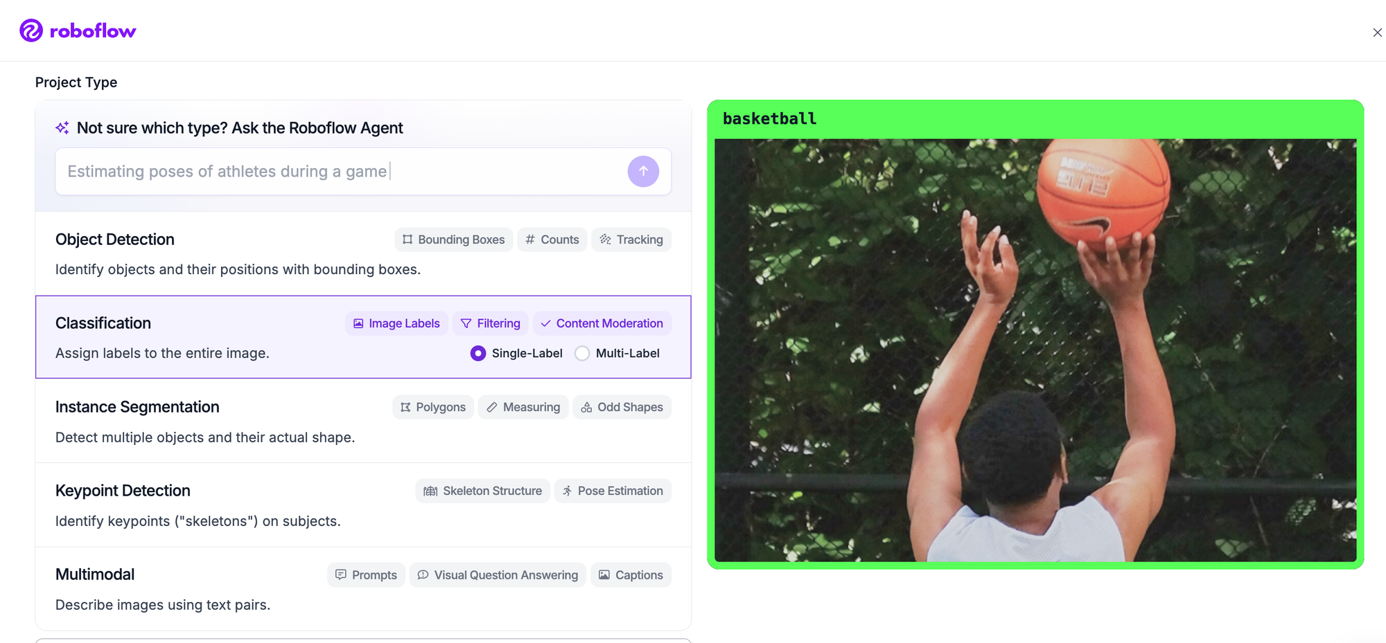
Sign in to Roboflow, create a new project, and set the project type to Classification. Choose single-label if each image belongs to exactly one class (daisy or dandelion), or multi-label if an image can carry more than one tag. Name your classes.

Step 2: Add your images

Upload your images, grouped by class. If you want a head start, Roboflow Universe hosts a large library of open datasets you can fork, and the flowers dataset used here is available there. If your images are not yet sorted into classes, you can label them in the next step.

Step 3: Label your images

For classification, a label is the class assigned to the whole image rather than a box. You can assign classes in the Roboflow interface, or automate the first pass: Autodistill uses a foundation model like CLIP to label an unlabeled image folder from a short list of text prompts, so you review and correct instead of sorting every image by hand. Consistent labels are the biggest lever on final accuracy.

Step 4: Generate a dataset version

A version freezes your labeled images together with preprocessing and augmentation, and Roboflow auto-splits them into train, validation, and test sets. Resize is worth applying to standardize input dimensions. Augmentation is especially effective for classification: brightness, contrast, rotation, and noise all expand a small dataset and reduce overfitting, and you apply them with a click rather than a script. Keep your validation and test sets clean so your accuracy numbers reflect real images.

Step 5: Train your model

Open Roboflow Custom Training and start a classification training job. Classification models train from an ImageNet-pretrained checkpoint, so the network begins with broad visual knowledge and only has to learn your classes. This is transfer learning, and it is why a few hundred images per class is often enough. Training runs in the cloud, so there is nothing to install and no GPU to rent, and you get an email when it finishes.

Step 6: Evaluate your model

When training completes, Roboflow reports accuracy on the held-out test set along with a confusion matrix that shows which classes get mixed up. Read the per-class results, not just the overall number: two visually similar classes like daisy and dandelion are exactly where a classifier stumbles. If a class underperforms or a pair keeps getting confused, add or relabel examples for it and retrain. Two or three of these passes is what moves a model from promising to production-ready.

Step 7: Build a classification Workflow

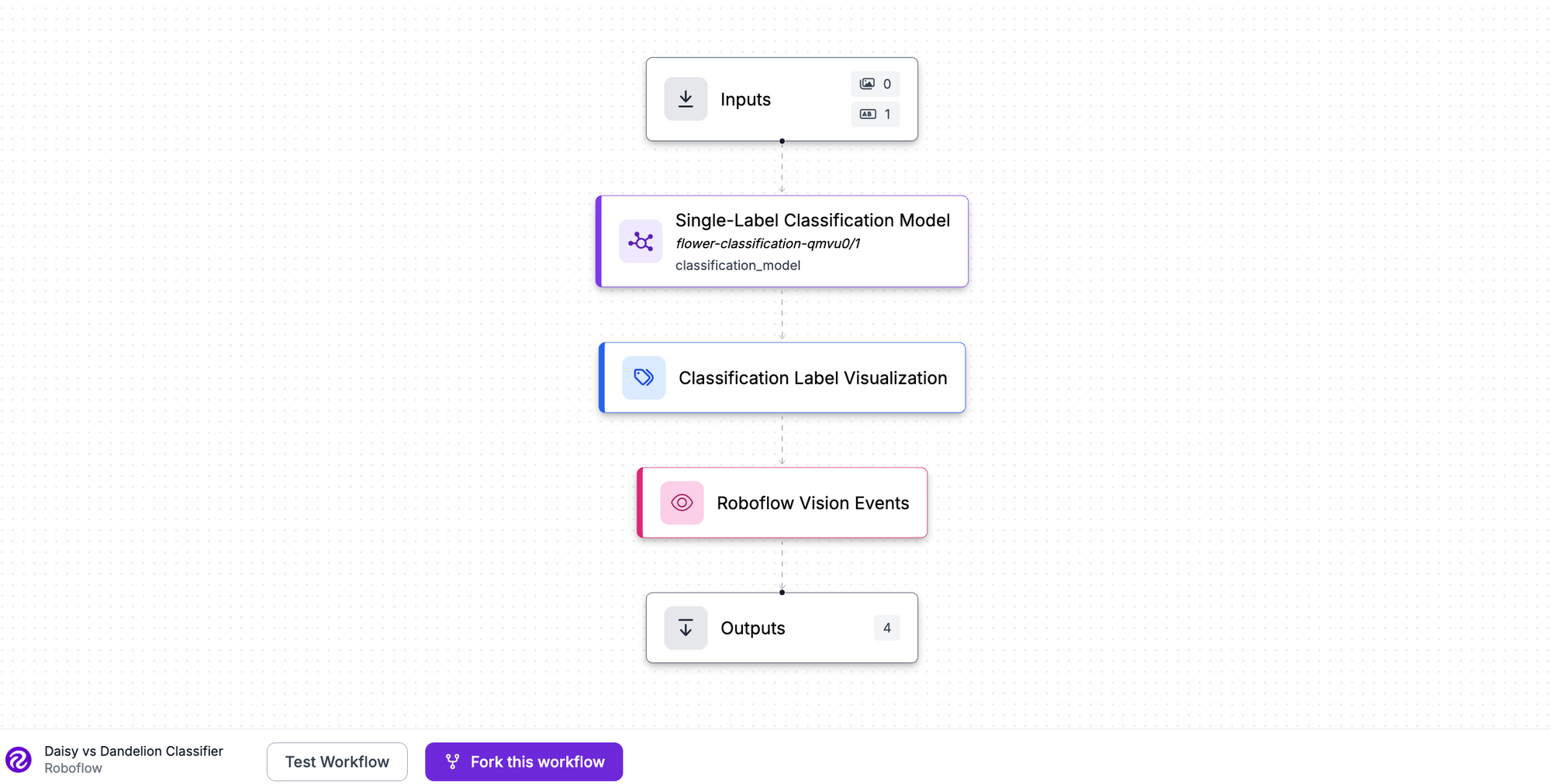
To turn the trained model into something you can run and act on, assemble it into a Roboflow Workflow, a low-code visual builder where you chain blocks into an application. For the flower classifier, the Workflow is four blocks:

An image input that receives the picture to classify.

A Single-Label Classification Model block pointed at your trained model (in our daisy versus dandelion example, our model is flower-classification-qmvu0/1). It returns the predicted class and a confidence score.

A Classification Label Visualization block that renders the predicted label onto the image, so the result is readable at a glance rather than buried in JSON.

A Roboflow Vision Events block that fires an event from each prediction, so a downstream system like a dashboard, a log, or an alert can react to what the model saw.

The Workflow returns the predicted class, the confidence, the annotated image, and the event.

Here's the workflow.

Step 8: Deploy and run the Workflow

Run the Workflow without standing up infrastructure. The Serverless Hosted API serves it behind an endpoint you can call from any language, and Roboflow Inference, the open source engine, runs it on-prem or on edge devices like NVIDIA Jetson, which suits the smaller, faster classifiers that real-time and on-device use call for.

You send an image and get back the predicted class and confidence, the annotated image, and any Vision Event the prediction triggered. Because the logic lives in the Workflow, you can add a confidence threshold or route a class to a different action without touching your application code.

If you work with a coding agent, the Roboflow MCP server connects your workspace to tools like Claude Code, Codex, and Cursor.

Build the Workflow with Roboflow Agent

If you would rather not add each block by hand, Roboflow Agent builds the Workflow for you from a plain text description. Instead of dragging blocks onto the canvas, you type what you want the pipeline to do, and the Agent assembles and connects the blocks, updating the canvas as it goes. For the flower classifier, a prompt as simple as this is enough to get started:

"Classify each image as daisy or dandelion with my classification model, draw the predicted label on the image, and send a vision event with the result."

From there you can keep refining in the same chat: ask it to only fire the event when confidence is above a threshold, or to route one class to a different action. It is the same Workflow either way, so you can start with the Agent and still open the canvas to adjust any block by hand.

Why Train a Classifier in Roboflow?

VGG-16 made the case that a deep network pretrained on ImageNet transfers well to new classification tasks. Roboflow gives you that benefit without the parts that make the original hard to reproduce. There is no framework to pin to an old version, no notebook that expires, and no GPU environment to match.

You label, generate a version, and train from an ImageNet checkpoint in the browser, then deploy to the cloud or the edge from the same place, so the whole path from images to a running classifier lives in one platform.

Can I still train the VGG-16 model in Roboflow?

Roboflow's hosted classification training uses an ImageNet-pretrained checkpoint rather than VGG-16 specifically, since newer architectures reach higher accuracy at lower cost. If you need the exact VGG-16 architecture, you can label and export your dataset from Roboflow in a standard format and train VGG-16 in your own environment, then bring the model back for deployment.

Is the VGG-16 model still good in 2026?

It still works and still posts strong accuracy, but at roughly 138 million parameters it is heavy and slower than modern options. For most new projects, a Vision Transformer or a ResNet gives better accuracy for the compute, and MobileNet is the usual choice when the model has to run in real time or on device.

What is the VGG-16 model used for?

Image classification is its main use, deciding which class an image belongs to. Because it produces strong general-purpose features, VGG-16 is also used for transfer learning and as a feature extractor, and its intermediate layers are a common choice for perceptual loss in image generation tasks.

What is the difference between VGG-16 and ResNet?

Both are deep convolutional classifiers, but ResNet adds residual (skip) connections that let information bypass layers, which makes very deep networks easier to train and generally more accurate and efficient than VGG-16 at a given depth. VGG-16 is simpler and more uniform, which is partially why it remains a popular teaching reference.

How much data do I need to train a classifier?

With transfer learning from an ImageNet checkpoint, a few hundred labeled images per class is often enough to get a working model. Start small, check the per-class accuracy and the confusion matrix, and add images for the classes that lag.

VGG16 Model: Get Started

You can train an image classification model on your own images today, entirely in the browser, and have a deployable model in an afternoon. Create a free Roboflow account and start with your own images or a dataset from Universe.

Cite this Post

Use the following entry to cite this post in your research:

Erik Kokalj. (Feb 25, 2026). How to Train a VGG-16 Image Classification Model on Your Own Dataset. Roboflow Blog: https://blog.roboflow.com/how-to-train-a-vgg-16-image-classification-model-on-your-own-dataset/