
This tutorial builds an inventory monitoring pipeline that extracts video frames at defined time intervals, runs each frame through Roboflow Inference Server against a model trained on packaged shelf items, and outputs structured CSV files (per-object detections, counts per interval, counts by class) along with bar charts showing detection patterns over time. The same pattern applies beyond retail shelves: any scenario where you need a time-stamped record of what a camera sees, from warehouse receiving to security anomaly detection, benefits from this interval-based sampling and structured export approach.
Real-time insights extracted from video streams can drastically improve efficiency for how industries operate. One high-impact application of this is in inventory management. Whether you’re a factory manager looking to improve inventory management or a store owner striving to prevent stockouts, real-time data can be a game-changer.
This tutorial will walk you through how to use computer vision to analyze video streams, extract insights from video frames at defined intervals, and present these as actionable visualizations and CSV outputs.
Inventory Management AI
Here is the output of the application we will build for detecting the objects from the videos:
By the end, you'll have detailed visualizations and CSV outputs of detected objects. You can read about what each visuals represent at the end of the blog.
object_counts_by_class_per_interval.csv
object_counts_per_interval.csv
predictions.csv
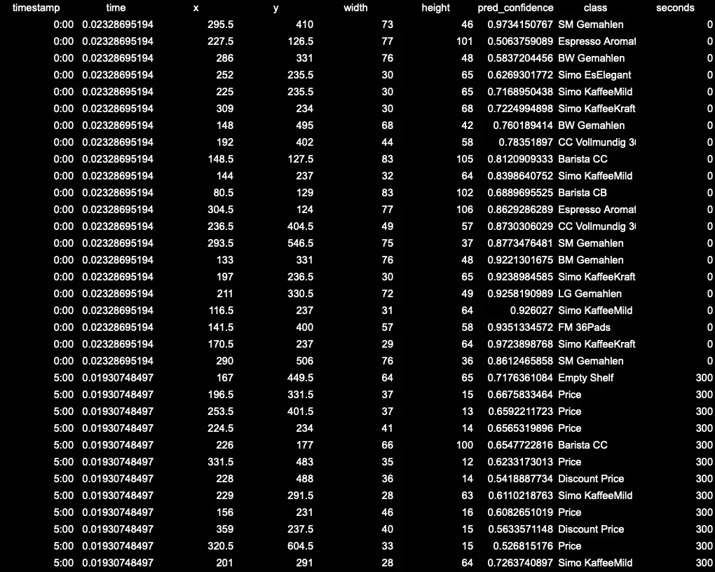
- timestamp: Refers to the time interval at which a frame was extracted from the video.
- time: Refers to the time the API took to process and return predictions for the frame. This is usually in terms of milliseconds and helps in understanding the performance of the API.
To build a dashboard with inference server, we will:
- Install the dependencies
- Extract frames at intervals
- Get predictions using inference server
- Visualize the result
We'll be working with an image dataset that are packaged coffee items on shelves and utilizing a model trained on those inventory items.
We will be deploying the model using the Roboflow Inference Server, an inference server in this case is used to deploy, manage, and serve machine learning models for inference in a production environment. Once a machine learning model has been trained using a dataset, it's not enough to just have the model – you need a way to use it, especially in real-time applications. That's where the inference server comes in.
It's also important to grasp that these predictions are essentially samples of data and you'll want to create the right environment to capture data at consistent intervals, which then can be time stamped and used for analysis, alerts, or as an input to other applications.
Step #1 Install the dependencies
Before we can start building our dashboard, we need to ensure you have your environment set up. Depending on if you are going to be using CPU or GPU, we run different kinds of dockerfiles. To optimize performance, it is a good idea to use GPU for the inference. For more info, you can look at our doc.
1. Run the inference server
- For systems with x86 CPU:
docker run --net=host roboflow/roboflow-inference-server-cpu:latest- For systems with NVIDIA GPU:
docker run --network=host --gpus=all roboflow/roboflow-inference-server-gpu:latestWith the required dependencies installed, we are now ready to start building our dashboard. Start by importing the required dependencies for the project:
import cv2
import pandas as pd
import pickle
import requests
import matplotlib.pyplot as plt
import os
Now, let’s start working on the main code for our dashboard.
Step #2 Extract Frames at Intervals
We are going to get frames from a given video at regular intervals and save them in frames array. Let’s define a function that extracts the frames at specific time intervals:
def extract_frames(video_path, interval_minutes):
    cap = cv2.VideoCapture(video_path)
    frames = []
    timestamps = []
    fps = int(cap.get(cv2.CAP_PROP_FPS))
    frame_count = 0

    while cap.isOpened():
        ret, frame = cap.read()
        if not ret:
            break
        if frame_count % (fps * interval_minutes) == 0:
            frames.append(frame)
            timestamps.append(frame_count / fps)
        frame_count += 1
    cap.release()
    return frames, timestamps
Step #3 Get Predictions using Inference Server
Using the frames we extracted, let’s use the fetch_predictions function to send each extracted frame to our inference server.
We use the fetch_predictions function to interact with our inference server. Simply put, for each image frame, the function sends it to our API, which then returns predictions about objects in the frame. These predictions, along with their timestamps, are organized into a table, ensuring you can quickly review results in chronological order. It's all about streamlining the process of getting insights from our images!
def fetch_predictions(base_url, frames, timestamps, dataset_id, version_id, api_key, confidence=0.5):
    headers = {"Content-Type": "application/x-www-form-urlencoded"}
    df_rows = []
    for idx, frame in enumerate(frames):
        numpy_data = pickle.dumps(frame)
        res = requests.post(
            f"{base_url}/{dataset_id}/{version_id}",
            data=numpy_data,
            headers=headers,
            params={"api_key": api_key, "confidence": confidence, "image_type": "numpy"}
        )
        predictions = res.json()

        for pred in predictions['predictions']:
            time_interval = f"{int(timestamps[idx] // 60)}:{int(timestamps[idx] % 60):02}"
            row = {
                "timestamp": time_interval,
                "time": predictions['time'],
                "x": pred["x"],
                "y": pred["y"],
                "width": pred["width"],
                "height": pred["height"],
                "pred_confidence": pred["confidence"],
                "class": pred["class"]
            }
            df_rows.append(row)

    df = pd.DataFrame(df_rows)
    df['seconds'] = df['timestamp'].str.split(':').apply(lambda x: int(x[0])*60 + int(x[1]))
    df = df.sort_values(by="seconds")
    return df
Step #4 Visualize the Result
This function turns your data into bar charts and saves them as image files.
def plot_and_save(data, title, filename, ylabel, stacked=False, legend_title=None, legend_loc=None, legend_bbox=None):
    plt.style.use('dark_background')
    data.plot(kind='bar', stacked=stacked, figsize=(15,7))
    plt.title(title)
    plt.ylabel(ylabel)
    plt.xlabel('Timestamp (in minutes:seconds)')

    if legend_title:
        plt.legend(title=legend_title, loc=legend_loc, bbox_to_anchor=legend_bbox)

    plt.tight_layout()
    plt.savefig(filename)
Putting It All Together
The main function shows the entire pipeline:
- First, we Initialize: Set up constants like the base URL, video path, dataset ID, and API key.
- Then, we extract frames: Extract frames from the video at specified intervals using extract_frames.
- We fetch predictions: Use the fetch_predictions function to obtain object predictions for each frame from the inference server and save the predictions in a CSV format within a results directory.
- Finally, we visualize: Plot the overall count of detected objects over time using plot_and_save and group and plot object detections by class over time.
Execute the script, and the results are automatically processed, stored, and visualized.
def main():
base_url = "http://localhost:9001"
video_path = "video_path"
dataset_id = "dataset_id"
version_id = "version_id"
api_key = "roboflow_api_key"
interval_minutes = args.interval_minutes * 60
frames, timestamps = extract_frames(video_path, interval_minutes)
df = fetch_predictions(base_url, frames, timestamps, dataset_id, version_id, api_key)
if not os.path.exists("results"):
os.makedirs("results")
#saving predictions response to csv
df.to_csv("results/predictions.csv", index=False)
# Transform timestamps to minutes and group
df['minutes'] = df['timestamp'].str.split(':').apply(lambda x: int(x[0]) * 60 + int(x[1]))
object_counts_per_interval = df.groupby('minutes').size().sort_index()
object_counts_per_interval.index = object_counts_per_interval.index.map(lambda x: f"{x // 60}:{x % 60:02}")
object_counts_per_interval.to_csv("results/object_counts_per_interval.csv")
# Quick insights
print(f"Total unique objects detected: {df['class'].nunique()}")
print(f"Most frequently detected object: {df['class'].value_counts().idxmax()}")
print(f"Time interval with the most objects detected: {object_counts_per_interval.idxmax()}")
print(f"Time interval with the least objects detected: {object_counts_per_interval.idxmin()}")
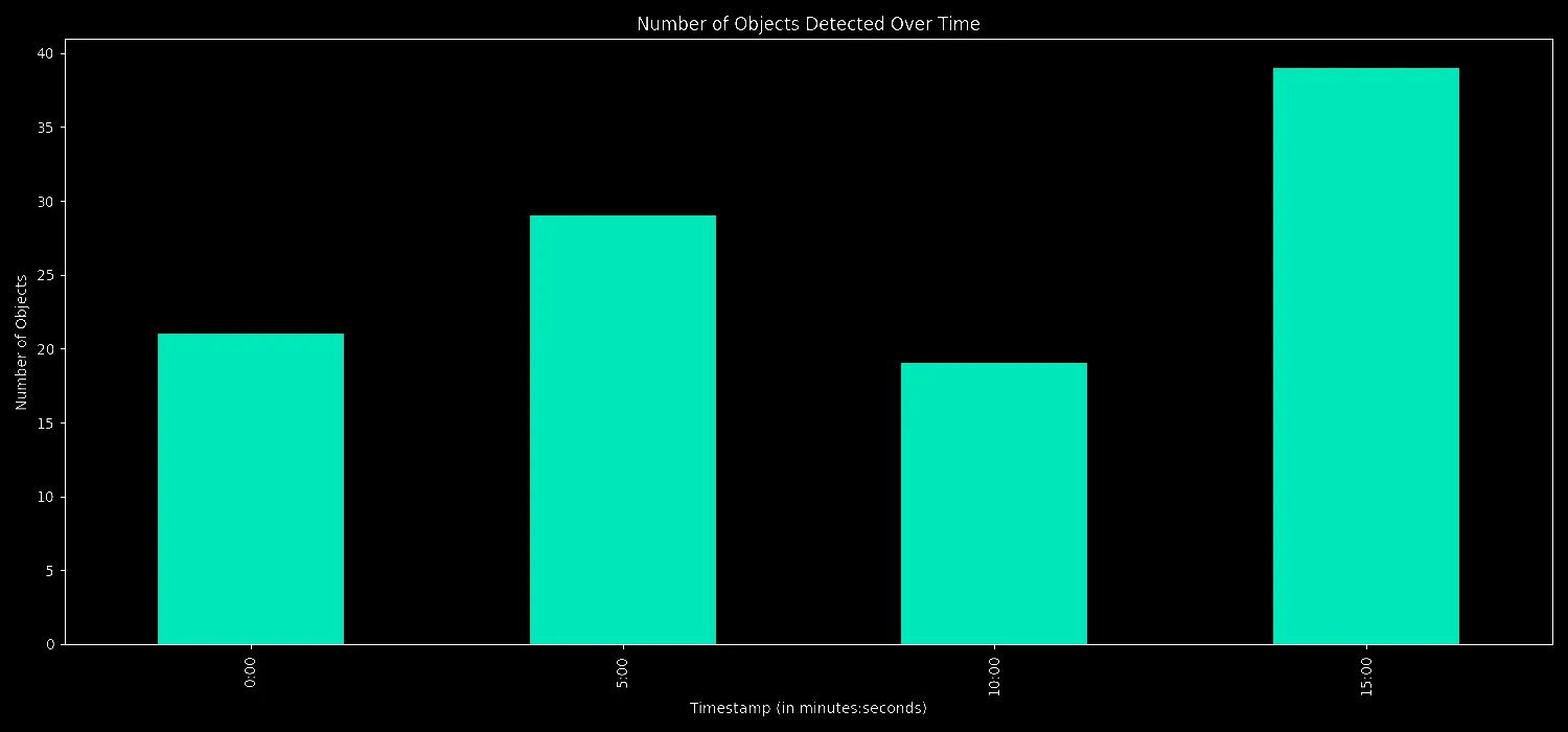
plot_and_save(object_counts_per_interval, 'Number of Objects Detected Over Time', "results/objects_over_time.png", 'Number of Objects')
# Group by timestamp and class, then sort by minutes
objects_by_class_per_interval = df.groupby(['minutes', 'class']).size().unstack(fill_value=0).sort_index()
objects_by_class_per_interval.index = objects_by_class_per_interval.index.map(lambda x: f"{x // 60}:{x % 60:02}")
objects_by_class_per_interval.to_csv("results/object_counts_by_class_per_interval.csv")
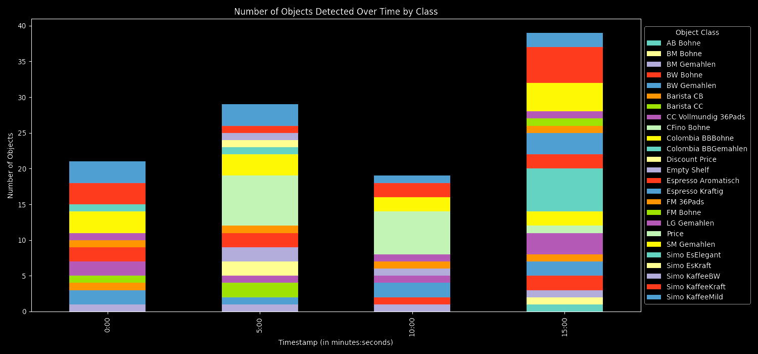
plot_and_save(objects_by_class_per_interval, 'Number of Objects Detected Over Time by Class', "results/objects_by_class_over_time.png", 'Number of Objects', True, "Object Class", "center left", (1, 0.5))
if __name__ == "__main__":
main()Running the Code Directly
Here's a quick rundown on how to get it up and running:
- Begin by cloning the inference dashboard example from GitHub:
git clone https://github.com/roboflow/inference-dashboard-example.git
cd inference-dashboard-example
pip install -r requirements.txt
2. Now, execute the main script with appropriate parameters:
python main.py --dataset_id [YOUR_DATASET_ID] --api_key [YOUR_API_KEY] --video_path [PATH_TO_VIDEO] --interval_minutes [INTERVAL_IN_MINUTES]
After running the script, head to the results folder to see the processed video data. Inside, you'll find:
predictions.csv: Holds specifics of every object detected, like where it's located, its size, and its type.object_counts_per_interval.csv: Gives a sum of all objects picked up within set time frames.object_counts_by_class_per_interval.csv: Lists how often each kind of object appears within those time frames.- Bar Charts: These graphs illustrate object detections over the video's duration, both as a total count and by individual object types.
Inventory Management AI
By extracting frames and analyzing them, it provides a summarized view of activity over time. The ability to categorize detections means you can discern patterns – perhaps certain objects appear more during specific periods. The insights can be applied across various fields, from detecting anomalies in security footage to understanding wildlife movements in recorded research data.
Learn more about using inventory management AI to improve your facilities' operations and reduce costs, when you talk to an AI expert.
Cite this Post
Use the following entry to cite this post in your research:
Arty Ariuntuya. (Aug 22, 2023). How to Use Computer Vision to Monitor Inventory: Inventory Management AI. Roboflow Blog: https://blog.roboflow.com/how-to-use-computer-vision-to-monitor-inventory/