
Every product that leaves a manufacturing line represents a promise of quality. Whether it is a smartphone, an automotive part, or a medical device, customers expect products to arrive free of defects. Even a small crack or missing component can result in wasted materials, production delays, and unhappy customers. As production lines become faster and produce more products, inspecting every item manually becomes increasingly difficult. Computer vision helps solve this problem by automating defect inspection while improving both speed and consistency. In this guide, we'll explore how computer vision powers modern defect inspection and build an automated defect inspection system using Roboflow.
What Is Defect Inspection?
Defect inspection is the process of identifying products that contain manufacturing defects before they move to the next stage of production or reach the customer. During inspection, each product is examined for flaws that prevent it from meeting predefined quality standards, such as cracks, missing components, incorrect dimensions, or cosmetic imperfections. The primary goal of defect inspection is to catch defects as early as possible, reducing scrap, minimizing costly product recalls, preventing production downtime, and ensuring that only high-quality products leave the factory.
Types of Manufacturing Defects
Not all manufacturing defects look the same. Depending on the product and production process, manufacturers may need to inspect for several different types of visual defects.
Surface defects: Surface defects are imperfections that appear on the outside of a product. Common examples include cracks, scratches, dents, corrosion, stains, and contamination. Because these defects are visible, they can be captured by a camera and identified by a computer vision model.
Dimensional defects: Dimensional defects happen when a part does not meet its required measurements or tolerances. For example, a hole may be drilled in the wrong location, a component may be too large or too small, or a bottle may be underfilled. Images captured by a camera can be analyzed to verify that a part meets its expected dimensions and quality standards.
Assembly defects: Assembly defects happen when components are missing, installed incorrectly, or misaligned during manufacturing. Examples include a missing resistor on a printed circuit board, a connector installed backwards, or a missing screw. A camera can capture the assembled product, allowing the inspection system to verify that all required components are present and correctly positioned.
Cosmetic defects: Cosmetic defects affect the appearance of a product without impacting how it functions. Examples include paint blemishes, misaligned labels, discoloration, fingerprints, wrinkles in packaging, and uneven finishes. Since these defects are visible, they can be captured by a camera and automatically identified during inspection.
Although these defects vary in appearance, they all share the same goal of inspection, identifying products that do not meet quality standards. Later on, we'll look at how different computer vision models can be used to detect each type of defect.
How Computer Vision Powers Modern Defect Inspection
Different types of defects require different computer vision models. Some defects can be detected by locating an object, while others require identifying precise boundaries or finding abnormalities that were never seen during training. Choosing the right approach depends on the type of defect being inspected and the level of detail required.
Object detection: Object detection identifies and localizes defects by drawing bounding boxes around them. This approach works well when defects have a clear location and appearance, such as missing components, dents, cracks, or damaged packaging. Models such as RF-DETR can detect multiple defects in a single image and return both their location and class.
Segmentation: Segmentation goes a step further by outlining the exact shape of a defect instead of drawing a bounding box around it. This is useful for defects with irregular shapes, such as cracks, corrosion, or scratches, where the size and precise boundaries of the defect are important. Models such as SAM 3 can generate detailed segmentation masks that make these defects easier to measure and analyze.
Anomaly detection: In some cases, it is difficult to collect examples of every possible defect. Instead of learning what defective products look like, anomaly detection models learn what normal products should look like and identify anything that appears unusual. This approach is useful for detecting rare or previously unseen defects that may not have been included in the training dataset.
Vision language models: Vision language models combine image understanding with natural language reasoning. After a defect has been detected, a model such as Gemini can analyze the affected region and generate a natural language explanation of the defect. For example, it can describe a missing component, explain why a product failed inspection, or generate a summary for a quality control report.
These models are often used together within a single inspection pipeline. For example, an object detection model such as RF-DETR can first locate a defect. The detected region can then be cropped and passed to a vision-language model such as Gemini, which can generate a description of the defect and summarize the inspection results. This allows manufacturers to automate both defect detection and reporting.
How to Build a Defect Inspection System
For this tutorial, we'll use PCB defect detection as a concrete example of how this pipeline comes together in practice. PCBs are a good fit because their defects are discrete, visually distinct, and localized, which makes them well suited to the detect-crop-classify pattern.
The same workflow structure applies to other inspection use cases too, whether that's checking welds on a metal part or verifying seal integrity on pharmaceutical packaging. We'll use a public dataset from Roboflow Universe, train a custom RF-DETR model on it, and wire everything into a Roboflow Workflow that detects each defect, crops in on it, classifies its type, and outputs a structured pass/fail result.
Step 1: Log Into Roboflow
Sign in to your Roboflow account to get started. If you don't have one yet, you can create a free account in just a few minutes. Once you're signed in, make sure you have a workspace set up, since that's where your datasets, models, and workflows will all live throughout this project.
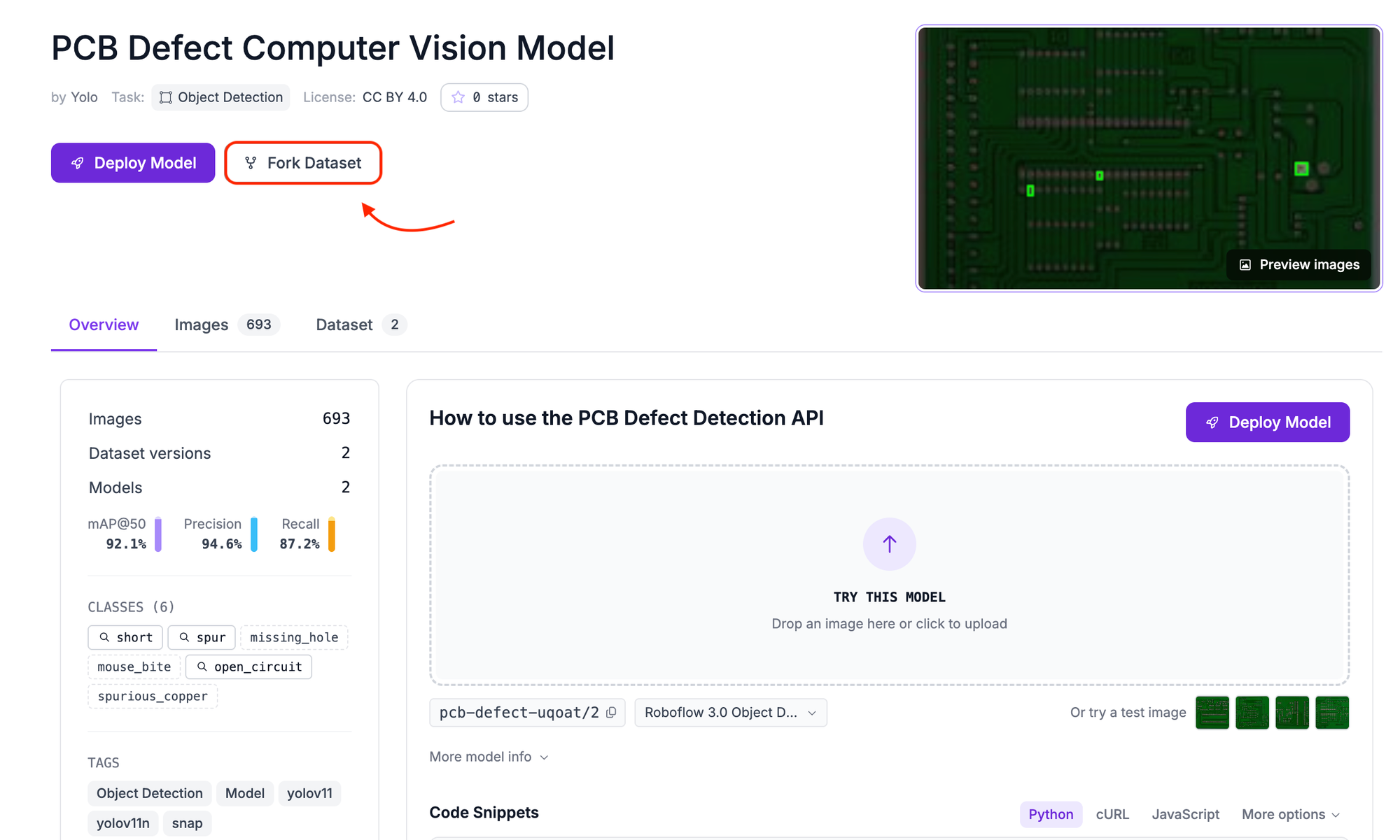
Step 2: Fork the Dataset from Roboflow Universe
Rather than collecting and annotating PCB images from scratch, we'll use an existing open-source dataset from Roboflow Universe. The dataset we'll use is the PCB Defect dataset, which contains 693 annotated images across six defect classes. Forking creates a private copy inside your workspace so you can apply your own preprocessing, augmentations, and split ratios without affecting the original.
To fork the dataset, open the dataset link in your browser. Click the Fork Dataset button in the top right corner of the page. Select your workspace as the destination. Click Fork Dataset once more to confirm, and Roboflow will copy all images and annotations into a new project in your workspace.
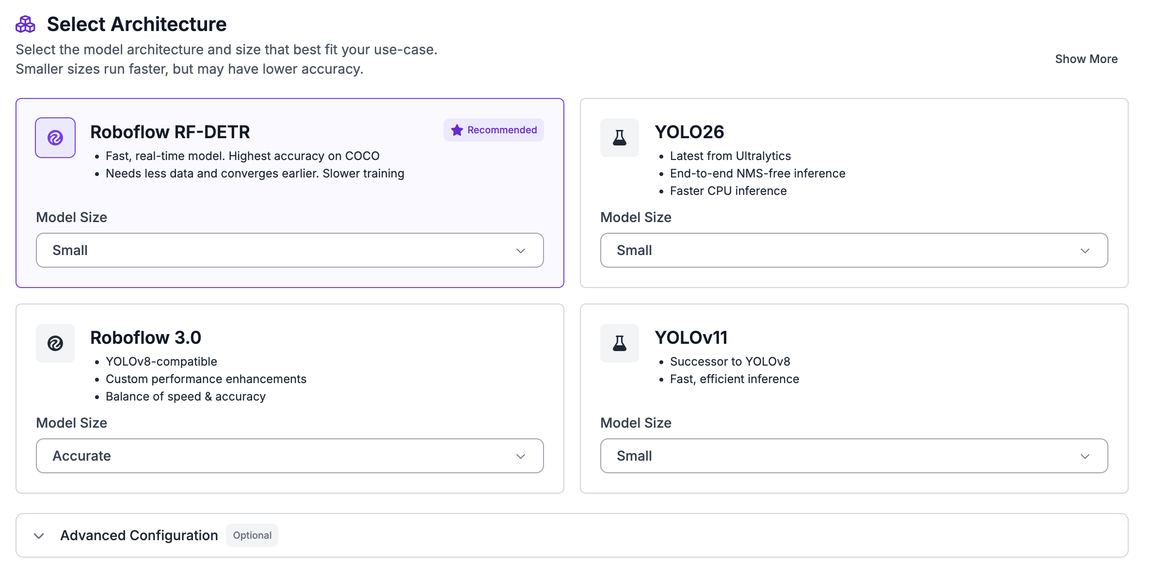
Step 3: Train an RF-DETR Model
Now that the dataset is in your workspace, it's time to train a detection model on it. Open your forked project and click the Train tab in the left sidebar. Select Custom Training as your training engine. When prompted to choose a model architecture, select RF-DETR from the list and set the model size to Small.
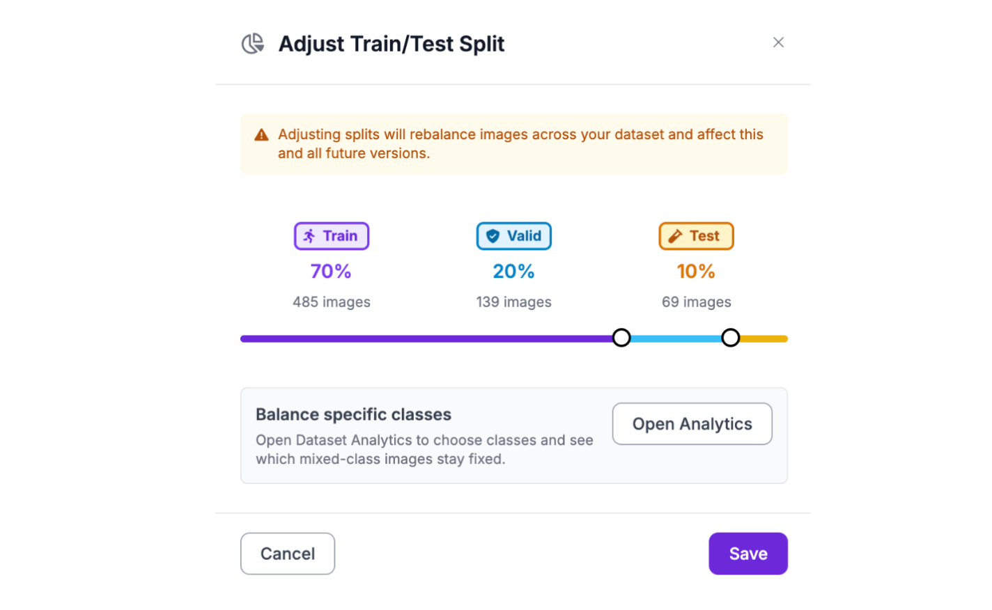
Step 4: Configure the Train/Validation/Test Split
Before Roboflow can start training, it needs a dataset version with a defined split across training, validation, and test sets. Each split serves a different purpose during the training process.
The training set is what the model actually learns from, so the more images here the better. The validation set is never used for learning, it's used after each epoch to check whether the model is improving or starting to overfit. The test set stays completely untouched until training finishes and gives you an honest, unbiased read on final model performance.
A standard split for a dataset of this size is 70% training, 20% validation, and 10% test. Roboflow lets you set these ratios when generating a new dataset version and will assign images automatically. If the forked dataset already has a split defined, Roboflow will respect it by default, but you can override it here.
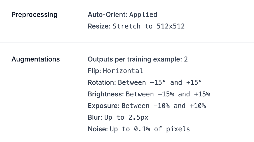
Step 5: Apply Preprocessing and Augmentation
With the split configured, the next step is to apply preprocessing and augmentation to your dataset version. These settings get baked into the dataset version you generate, so the model trains on consistently formatted, realistically varied images from the start.
For preprocessing, two steps are applied here. Auto-Orient corrects any rotation metadata embedded in images from different cameras, since a sideways PCB image will confuse the model during training. Resize (Stretch to 512×512) brings every image to a fixed resolution, which RF-DETR requires as a fixed input size.
For augmentation, the following settings are applied, with the output per training example set to 2. This generates one augmented variant for each original training image, doubling the size of the training dataset.
- Flip (Horizontal) helps the model handle boards imaged from either orientation
- Rotation (between -15° and +15°) accounts for slight camera misalignment on the inspection line
- Brightness (between -15% and +15%) and Exposure (between -10% and +10%) simulate the lighting variation you'll encounter in a real facility
- Blur (up to 2.5px) teaches the model to handle minor focus inconsistencies from a moving conveyor
- Noise (up to 0.1% of pixels) improves robustness against camera sensor noise
Once you've configured these, click Generate to create your dataset version and start training.
Step 6: Evaluate the Training Results
Once training completes, Roboflow will show you the evaluation results for your model against the test set. Here's what the trained PCB defect model achieved:
| Metric | Score |
|---|---|
| mAP@50 | 87.1% |
| Precision | 96.1% |
| Recall | 81.6% |
| F1 | 88.3% |
An 87.1% mAP@50 indicates that the model performs well across all six defect classes. The 96.1% precision score means that when the model identifies a defect, it is usually correct, resulting in very few false positives. The 81.6% recall score shows that the model successfully detects most defects, although some may still be missed. If your application prioritizes catching every possible defect, you can lower the confidence threshold in your Workflow to improve recall. Finally, the 88.3% F1 score shows that the model maintains a good balance between precision and recall.
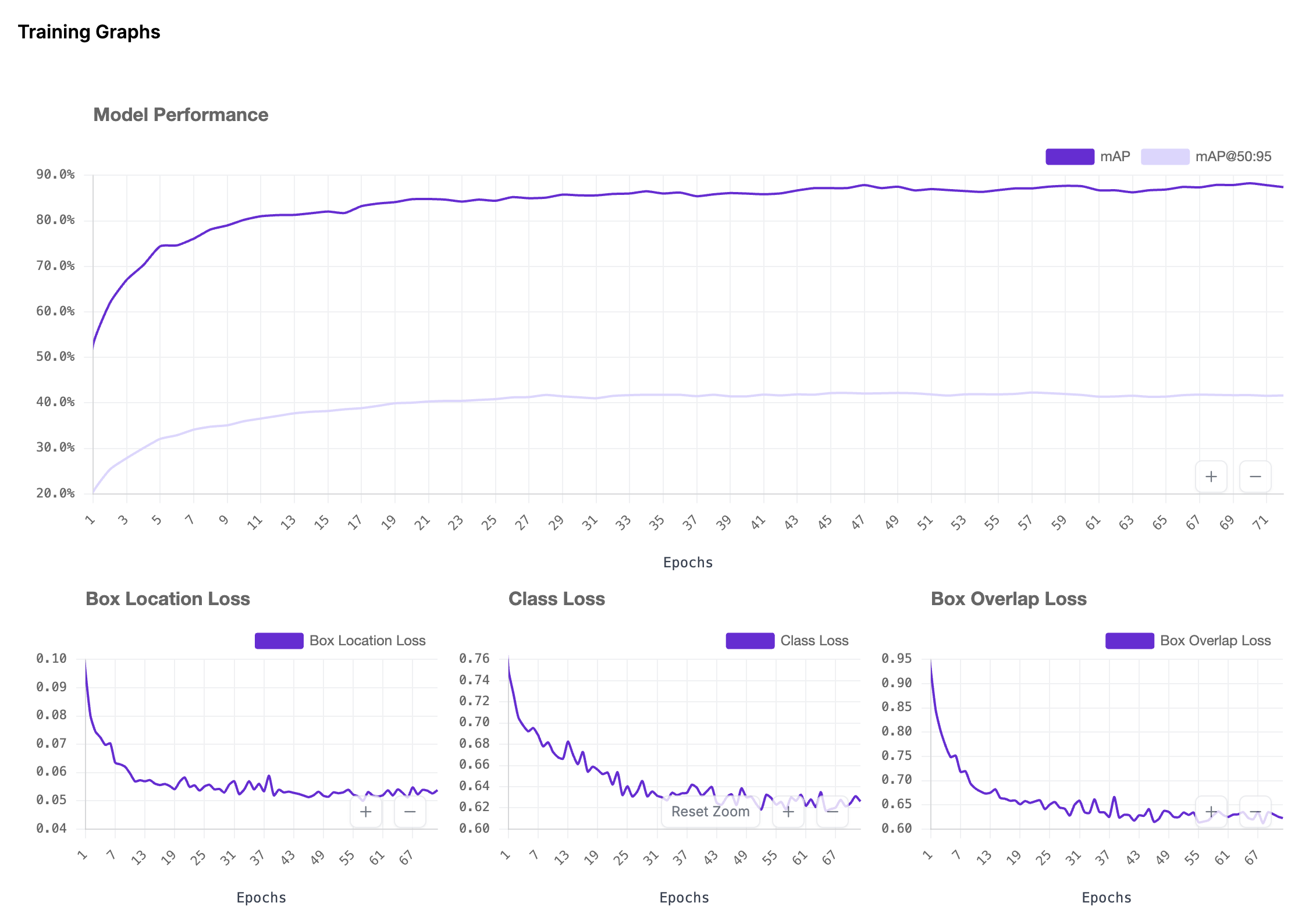
It's also worth reviewing the per class metrics after training. If one defect class performs noticeably worse than the others, it may need additional annotated examples before deployment.
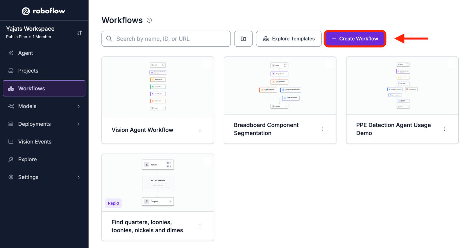
Step 7: Build the PCB Defect Inspection Workflow
Now that you have a trained model, it's time to wire it into an inspection pipeline. Navigate to the Workflows tab in your Roboflow dashboard and click Create Workflow.
Start from a blank canvas. The Image Input and Output blocks are already there by default, so we'll build everything in between. The first block we add after the Input will be the Object Detection Model, and we'll refer to that as the starting point of our pipeline. From there, the pipeline splits into two parallel branches, one handling the Gemini analysis and one handling the visualization, before coming back together at the Text Display block at the end.
Here's what the complete workflow looks like before we walk through each block.
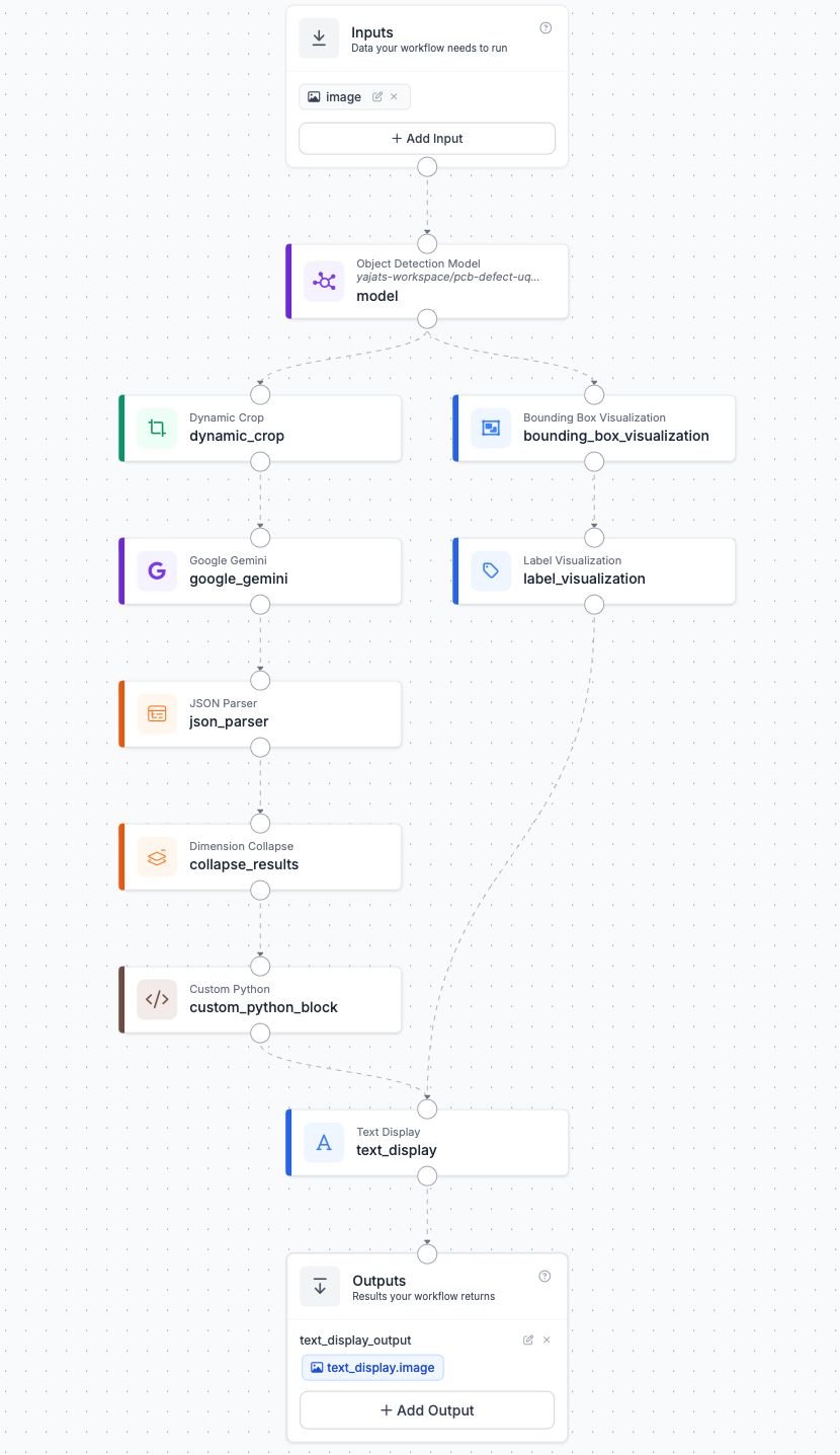
Block 1: Object Detection Model
The first block to add is the Object Detection Model. This is where your trained RF-DETR model runs on the incoming PCB image, returning a set of predictions, each containing a bounding box, class label, and confidence score for every defect it finds. Click Add Block and search for Object Detection Model. Connect it to the Image Input block. In the configuration panel, open the model dropdown and select your fine-tuned PCB defect model from your workspace.
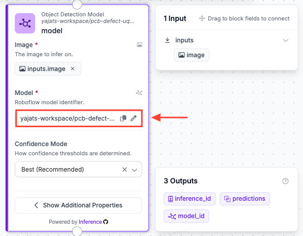
Since the model can find multiple defects on a single PCB, it returns a predictions array where each entry contains the bounding box coordinates, class label, and confidence score for a detected defect. The Dynamic Crop block in the left branch will then use these predictions to generate an individual crop for each one. The pipeline splits into two branches from here.
Left Branch: Gemini Analysis
This is where the actual inspection happens. Each defect detected by the model gets cropped out and sent to Gemini individually, which analyzes it and returns a pass or fail verdict. By the end of this branch, we'll have a single PASS/FAIL result and a count of the defects.
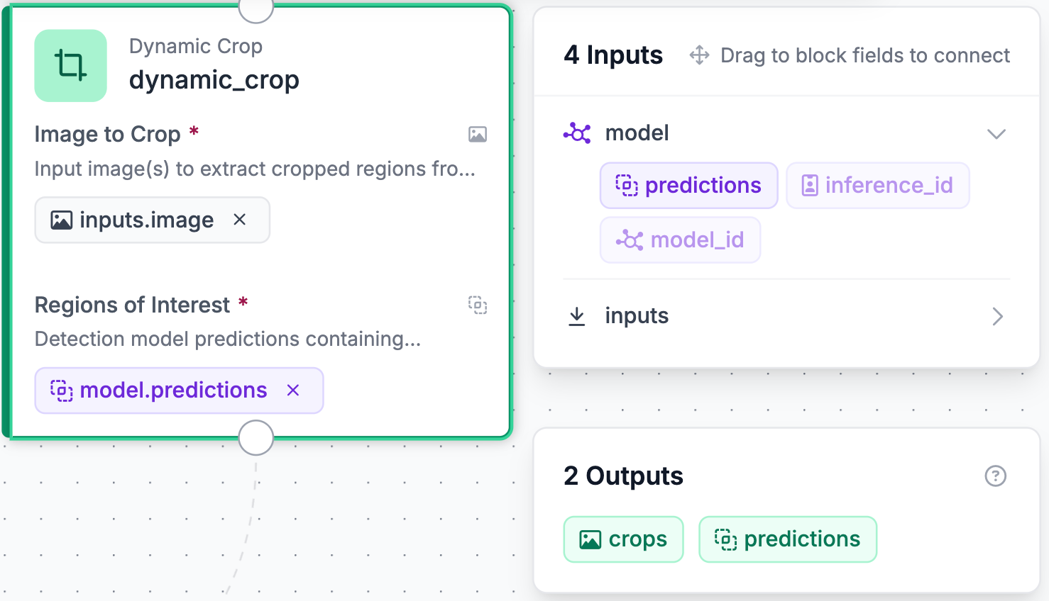
Block 2: Dynamic Crop
The left branch starts with the Dynamic Crop block. Rather than passing the full PCB image to Gemini, we crop tight on each individual detection first, since Gemini will reason much more accurately about a zoomed-in defect region than about a tiny bounding box on a large image. Click Add Block and search for Dynamic Crop. Connect it to the Object Detection Model block using the model's predictions as the crop input.
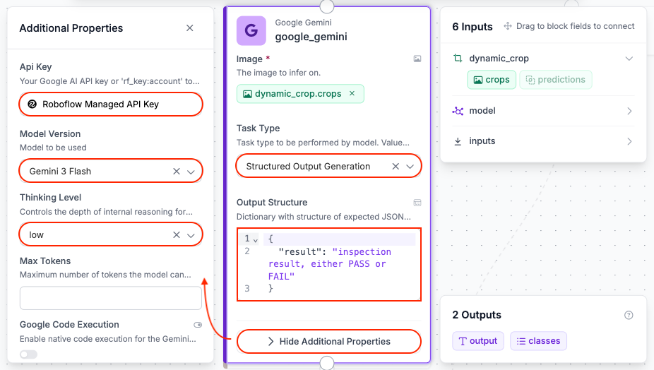
Block 3: Google Gemini
Next, add the Google Gemini block and connect it to the Dynamic Crop block, using dynamic_crop.crops as the image input. This is what analyzes each cropped defect region and returns a structured verdict. Configure it as follows:
- Task Type: Structured Output Generation
- Model Version: Gemini 3 Flash
- Thinking Level: low, since the decision here is straightforward and low thinking level keeps latency down
- API Key: Roboflow Managed API Key
- Output Structure — paste the following:
{
  "result": "inspection result, either PASS or FAIL"
}
In this workflow, Gemini acts as a verification layer on top of the RF-DETR detections, looking at each cropped defect region and confirming whether what the model found is actually a defect. That said, the workflow would work fine without it, too. Gemini just adds an extra layer of confidence that's worth the added latency for high-stakes inspection tasks.
Since Gemini runs on each crop independently, a PCB with four detected defects would produce four separate Gemini calls, one per crop, each returning its own PASS or FAIL verdict.
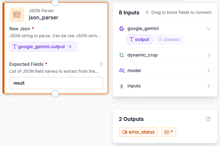
Block 4: JSON Parser
The JSON Parser block extracts the result from Gemini's raw text output and makes it available as an individual variable that downstream blocks can reference directly. Click Add Block, search for JSON Parser, and connect it to the Google Gemini block. Configure it like this:
- Raw JSON: Select
google_gemini.output - Expected Fields: Type
result
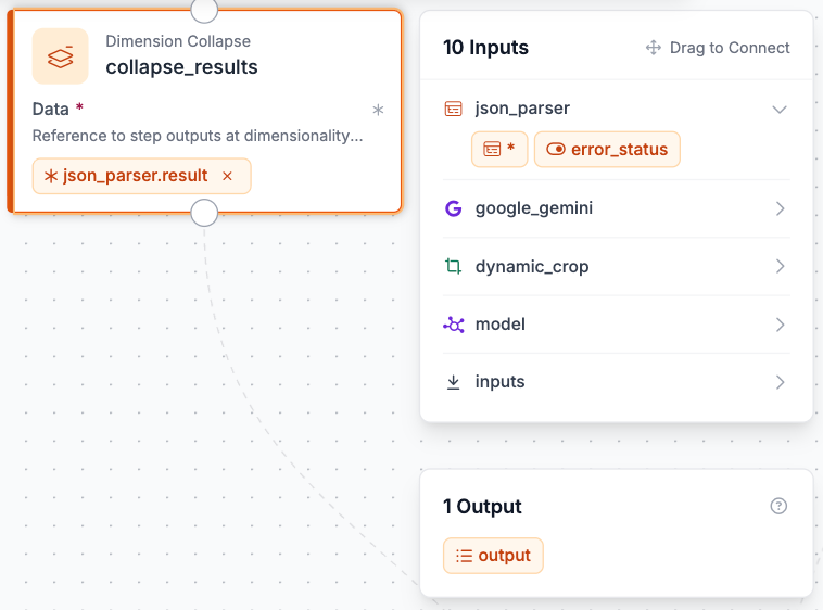
Block 5: Dimension Collapse
Since the Dynamic Crop block processes each detection individually, Gemini produces one PASS or FAIL result per crop rather than a single response for the whole board. The JSON Parser output at this point is therefore a nested list of individual results, one per crop. The Dimension Collapse block aggregates that nested list into a single flat output so the Custom Python block can iterate over all results at once. Without it, the Custom Python block would receive the data in the wrong format and fail. Click Add Block, search for Dimension Collapse, and connect it to the JSON Parser block.
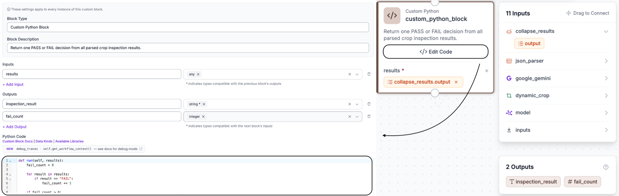
Block 6: Custom Python Block
This is where the PCB-level verdict gets calculated. Rather than evaluating each crop result individually, the Custom Python block looks across all of them and returns a single PASS or FAIL for the entire board, along with a count of how many defects failed. Click Add Block, search for Custom Python, and connect it to the Dimension Collapse block using collapse_results.output as the input. Configure the block with the following settings:
- Input name:
results, typeany - Output 1:
inspection_result, typestring - Output 2:
fail_count, typeinteger
Then paste the following code into the Python editor:
def run(self, results):
    fail_count = 0
    for result in results:
        if result == "FAIL":
            fail_count += 1
    if fail_count > 0:
        inspection_result = "FAIL"
    else:
        inspection_result = "PASS"
    return {
        "inspection_result": inspection_result,
        "fail_count": fail_count
    }
The logic is simple: it counts how many crops Gemini flagged as FAIL, and if that number is greater than zero the board fails. The fail_count gives the operator an immediate sense of how many defects were found rather than just a binary verdict.
Right Branch: Visualization
This branch takes the model predictions and draws annotated bounding boxes and labels onto the board image.
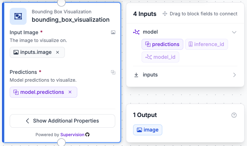
Block 2: Bounding Box Visualization
Now for the right branch, which handles what the operator actually sees. The Bounding Box Visualization block draws a bounding box around each defect detected by the model on the original board image. Click Add Block, search for Bounding Box Visualization, and connect it to the Object Detection Model block.
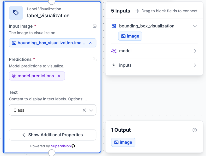
Block 3: Label Visualization
Right below the Bounding Box Visualization, add a Label Visualization block to overlay the defect class name on each bounding box. Connect it to the Bounding Box Visualization block so it draws on top of the already-annotated image.
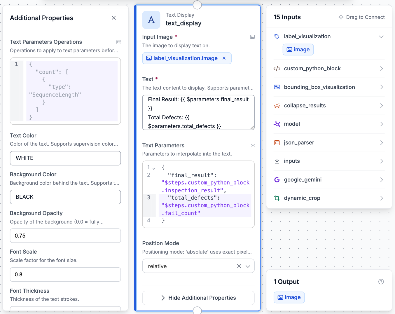
Block 4: Text Display
The final block brings both branches together. The Text Display block takes the annotated image from the Label Visualization and overlays the final result and defect count from the Custom Python block directly onto it. Click Add Block, search for Text Display, and configure it as follows:
- Input Image: select
label_visualization.image - Text — paste the following:
Final Result: {{ $parameters.final_result }}
Total Defects: {{ $parameters.total_defects }}
- Text Parameters — paste the following:
{
  "final_result": "$steps.custom_python_block.inspection_result",
  "total_defects": "$steps.custom_python_block.fail_count"
}
- Position Mode: Set to relative
This gives whoever is looking at the output everything they need at a glance: the annotated board image with each defect boxed and labeled, the overall PASS or FAIL verdict for the PCB, and a count of how many defects were found.
Click Save Workflow once all the blocks are connected. Your pipeline is ready to test.
Step 8: Test the Workflow
With all the blocks connected and the workflow saved, it's time to see it in action before deploying. Click the Test icon in the top right corner of the workflow editor and upload a PCB image to run through the pipeline.
Once the workflow finishes running, you'll see the final output image with bounding boxes drawn around each detected defect, class labels on each box, and the overall PASS or FAIL verdict along with the total defect count overlaid on the PCB. This is a good time to check that the result looks right and that Gemini is returning sensible verdicts before you push anything to production. If the output doesn't match what you'd expect, go back and adjust the confidence threshold on the Object Detection Model block and test again.
Step 9: Deploy the Workflow
Once you're satisfied with how the workflow is performing, click Deploy in the top right corner of the workflow editor. From the deployment options that appear, select Cloud Hosted API. Roboflow will generate the code you need to call your workflow from your own application.
Start by installing the Roboflow inference SDK:
pip install -U inference-sdkThen use the generated code to connect to your deployed workflow and run inference on an image:
python
from inference_sdk import InferenceHTTPClient

client = InferenceHTTPClient(
    api_url="https://serverless.roboflow.com",
    api_key="YOUR_API_KEY"
)

result = client.run_workflow(
    workspace_name="YOUR_WORKSPACE",
    workflow_id="YOUR_WORKFLOW_ID",
    images={
        "image": "YOUR_IMAGE.jpg"
    },
    use_cache=True
)

print(result)
Replace YOUR_API_KEY, YOUR_WORKSPACE, YOUR_WORKFLOW_ID, and YOUR_IMAGE.jpg with your own values. Running the script sends the image to your deployed workflow and returns the inspection result, defect count, and annotated output image.
If you'd prefer to keep everything on your own hardware rather than sending images to the cloud, select Self-Hosted API from the deployment options instead. Roboflow will walk you through installing Roboflow Inference and starting a local inference server, after which the workflow runs entirely on your own infrastructure with no data leaving your facility.
Defect Inspection Deployment Options
Once a defect inspection system has been tested, it can be deployed in different environments depending on the requirements of the production line.
Cloud deployment: In a cloud deployment, images are sent to a remote server where the computer vision model performs inference and returns the results. This approach makes it easy to scale inspection across multiple production lines and manage model updates from a central location. However, it depends on a reliable network connection and may introduce additional latency.
Edge deployment: Edge deployment runs the model on hardware located near the production line. Since inference happens locally, images do not need to leave the facility. This reduces latency, improves reliability, and helps protect sensitive manufacturing data. Edge deployment is a common choice for real-time inspection systems where fast decisions are required.
Offline deployment: Some manufacturing facilities operate on air gapped networks that are completely isolated from the internet for security or regulatory reasons. In these environments, the entire inspection system runs locally without any external connectivity. Offline deployment allows manufacturers to perform automated defect inspection while meeting strict security and compliance requirements.
After a defect has been detected, the inspection result often needs to trigger an action on the production line. For example, a defective product might be removed from the conveyor belt, an operator might receive an alert, or the inspection result might be logged for quality control. To make this possible, defect inspection systems are often integrated with factory equipment such as PLCs and HMIs. These systems commonly communicate using industrial protocols such as MQTT and OPC UA, allowing inspection results to become part of the broader manufacturing process.
Defect Inspection Conclusion
In this guide, we built a defect inspection system using Roboflow and explored how computer vision can automate quality inspection in modern manufacturing. Along the way, we covered the different types of manufacturing defects, compared manual and automated inspection, and learned when to use object detection, segmentation, anomaly detection, and vision language models for different inspection tasks.
Although this tutorial focused on building a general purpose defect inspection system, the same workflow can be adapted to a wide range of manufacturing applications. Whether you are inspecting printed circuit boards in electronics, verifying pharmaceutical packaging, detecting defects during automotive manufacturing, or identifying damaged packaging on a production line, computer vision provides a fast and scalable way to automate quality inspection. You can learn more about these applications in Roboflow's guides on electronics inspection, pharmaceutical inspection, and automotive inspection.
Ready to build your own defect inspection system? Get started with Roboflow and begin building computer vision workflows for your own manufacturing applications.
Cite this Post
Use the following entry to cite this post in your research:
Yajat Mittal. (Jul 1, 2026). Defect Inspection. Roboflow Blog: https://blog.roboflow.com/defect-inspection/