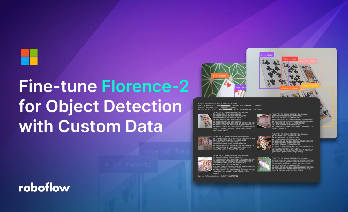
Florence-2 is a lightweight vision-language model open-sourced by Microsoft under the MIT license. The model demonstrates strong zero-shot and fine-tuning capabilities across tasks such as captioning, object detection, grounding, and segmentation. You can learn more about the capabilities of the pre-trained Florence model from our blog post.
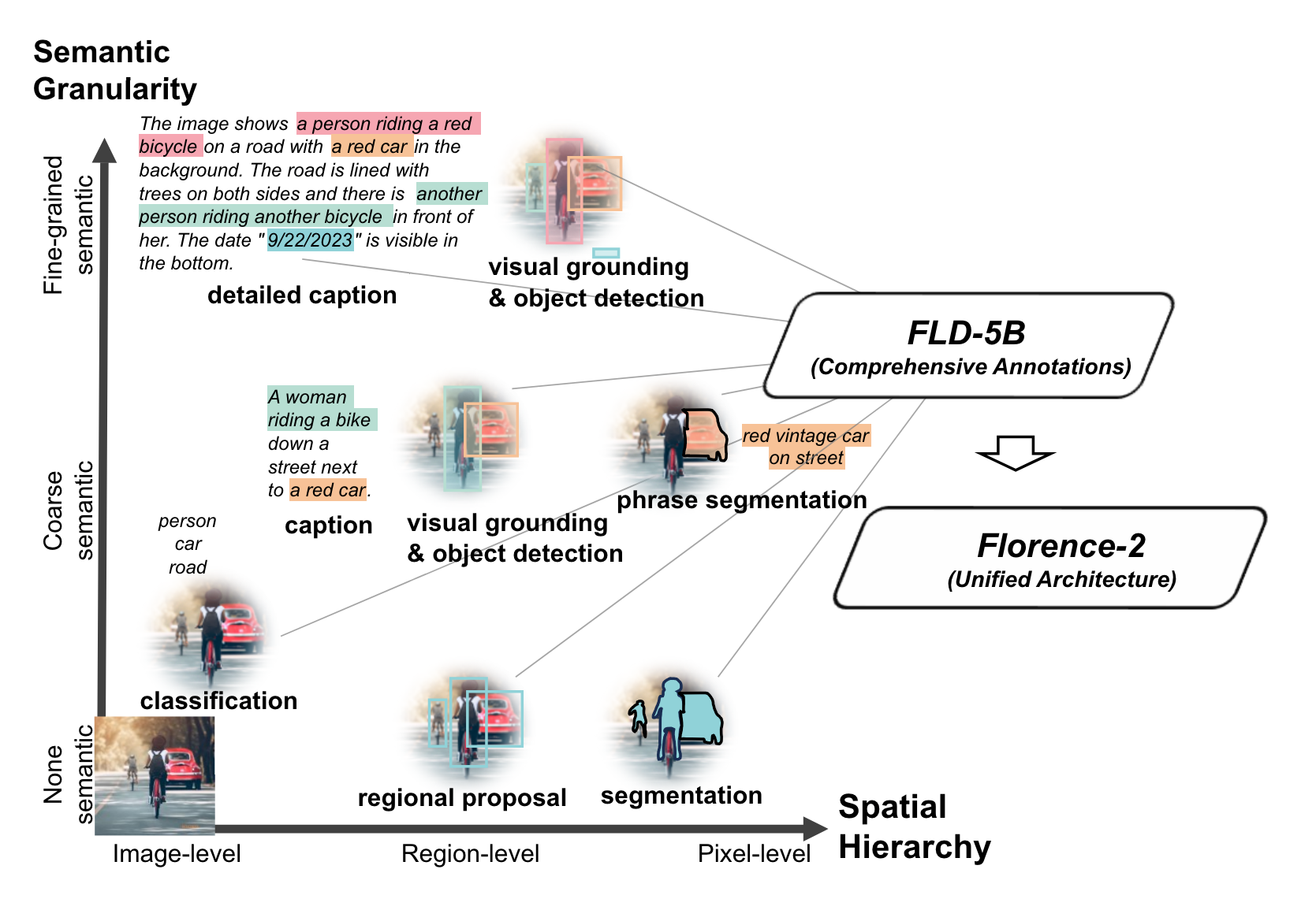
Like other pre-trained foundational models, Florence-2 may lack domain-specific knowledge. For example, it may perform poorly with medical or satellite imagery. In such cases, fine-tuning with a custom dataset is necessary. This tutorial will show you how to fine-tune Florence-2 on object detection datasets to improve model performance for your specific use case.
Let's dive in!


Getting Started
Before we fine-tune the Florence-2 model on a custom detection dataset, we need to properly configure our environment. This tutorial is accompanied by a notebook that you can open in a separate tab and follow along.
Before we discuss the data format, model training, and evaluation, make sure your environment is GPU-accelerated. If you are using our Google Colab, ensure you have access to an NVIDIA L4 GPU by running the nvidia-smi command. If you encounter any issues, navigate to Edit -> Notebook settings -> Hardwar accelerator, set it to L4 GPU, and then click Save.
If you are running the code locally, you will also need an NVIDIA GPU with approximately 20GB VRAM. Depending on the amount of memory on your GPU, you may need to choose different hyperparameter values during training, especially the batch size.
Additionally, we will need to set the values of two secrets: the HuggingFace token, to download the pre-trained model, and the Roboflow API key, to download the object detection dataset.
Open your HuggingFace settings page, click Access Tokens, then New Token to generate a new token. To get the Roboflow API key, go to your Roboflow settings page, and click Copy settings. This will place your private key in the clipboard. If you are using Google Colab, go to the left pane and click on Secrets (🔑).
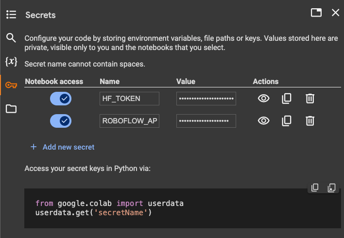
Then store the HuggingFace Access Token under the name HF_TOKEN and store the Roboflow API Key under the name ROBOFLOW_API_KEY. If you are running the code locally, simply export the values of these secrets as environment variables.
Florence-2 Dataset Format
In this example, I'll fine-tune Florence-2 on a dataset of poker cards - one of the datasets belonging to Roboflow 100. We'll use the roboflow package to download it.
from google.colab import userdata
from roboflow import Roboflow

ROBOFLOW_API_KEY = userdata.get('ROBOFLOW_API_KEY')
rf = Roboflow(api_key=ROBOFLOW_API_KEY)

project = rf.workspace("roboflow-jvuqo").project("poker-cards-fmjio")
version = project.version(4)
dataset = version.download("florence2-od")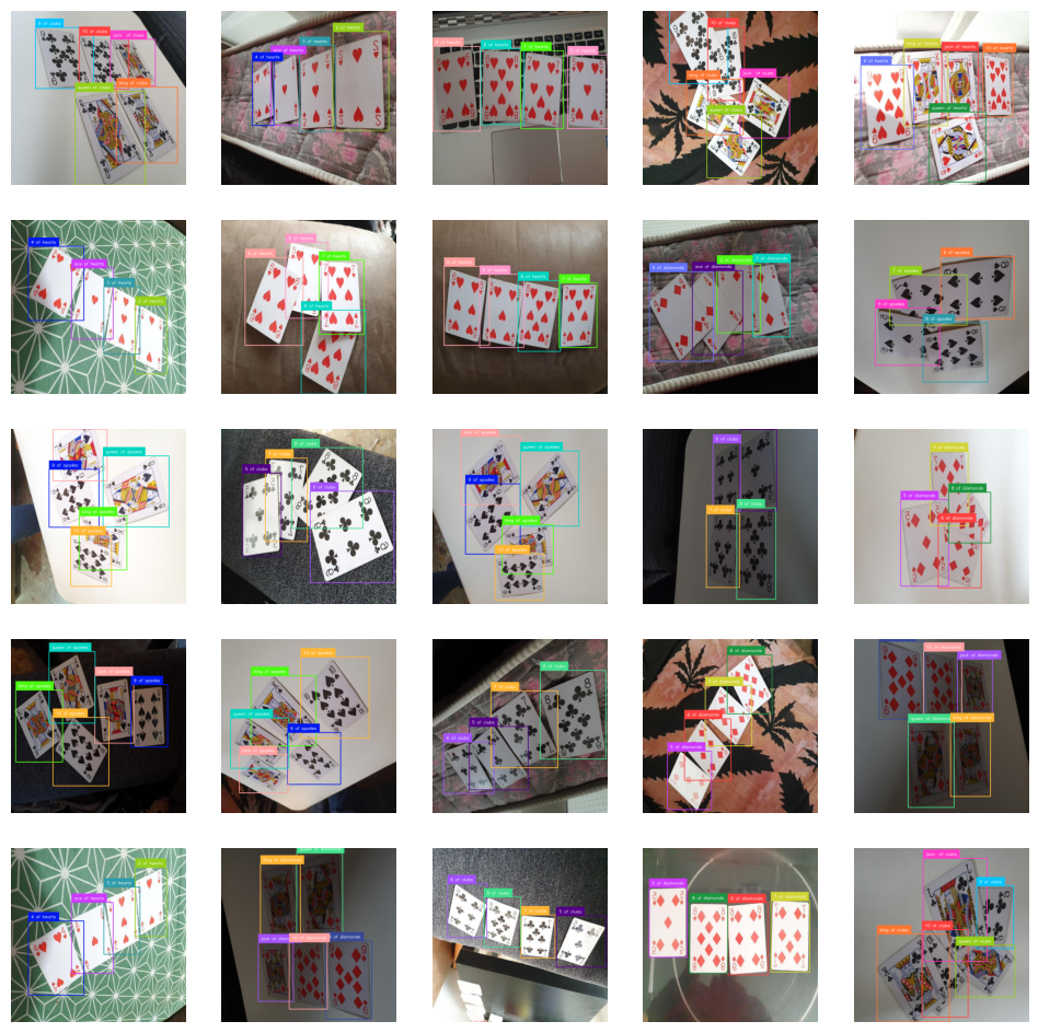
Each image must have a prefix and a suffix. For fine-tuning Florence-2 on an object detection task, the prefix (prompt) is always the same: <OD>. The suffix, the expected model response, has a structure similar to the one used in fine-tuning PaliGemma. Each bounding box is described by a string with the following structure: {class_name}<loc{x1}><loc{y1}><loc{x2}><loc{y2}>. Here, the values x1, y1, x2, y2 describe the coordinates of the bounding box vertices.
These values are first normalized (scaled to float values between 0 and 1 by dividing by the image resolution) and then multiplied by 1000 and rounded to integers. Ultimately, the values x1 y1, x2, y2 are integers in the closed range from 0 to 999.
{"prefix": "<OD>", "suffix": "10 of clubs<loc_142><loc_101><loc_465><loc_451>9 of clubs<loc_387><loc_146><loc_665><loc_454>jack of clubs<loc_567><loc_168><loc_823><loc_429>queen of clubs<loc_367><loc_467><loc_764><loc_998>king of clubs<loc_603><loc_440><loc_948><loc_871>", "image": "rot_0_7471_png_jpg.rf.30ec1d3771a6b126e7d5f14ad0b3073b.jpg"}
{"prefix": "<OD>", "suffix": "10 of clubs<loc_142><loc_101><loc_465><loc_451>9 of clubs<loc_387><loc_146><loc_665><loc_454>jack of clubs<loc_567><loc_168><loc_823><loc_429>queen of clubs<loc_367><loc_467><loc_764><loc_998>king of clubs<loc_603><loc_440><loc_948><loc_871>", "image": "rot_0_7471_png_jpg.rf.30ec1d3771a6b126e7d5f14ad0b3073b.jpg"}
{"prefix": "<OD>", "suffix": "10 of clubs<loc_142><loc_101><loc_465><loc_451>9 of clubs<loc_387><loc_146><loc_665><loc_454>jack of clubs<loc_567><loc_168><loc_823><loc_429>queen of clubs<loc_367><loc_467><loc_764><loc_998>king of clubs<loc_603><loc_440><loc_948><loc_871>", "image": "rot_0_7471_png_jpg.rf.30ec1d3771a6b126e7d5f14ad0b3073b.jpg"}
Load Pre-trained Florence-2 Model
Before we start fine-tuning the model on a custom dataset, we need to load the pre-trained Florence-2 model into memory. Florence-2 is available in two versions: base and large, with 230 million and 770 million parameters, respectively.
For this tutorial, we will use the base version. If you want to load the large version, remember that you will need more VRAM during training, or alternatively, reduce the batch size.
import torch
from transformers import AutoModelForCausalLM, AutoProcessor

CHECKPOINT = "microsoft/Florence-2-base-ft"
REVISION = 'refs/pr/6'
DEVICE = torch.device("cuda" if torch.cuda.is_available() else "cpu")

model = AutoModelForCausalLM.from_pretrained(
    CHECKPOINT, trust_remote_code=True, revision=REVISION).to(DEVICE)
processor = AutoProcessor.from_pretrained(
    CHECKPOINT, trust_remote_code=True, revision=REVISION)
After loading the model, we can test how it performs inference on a sample image. This step is not required, but a sample inference is a good way to confirm that our environment is configured correctly.
import supervision as sv
from PIL import Image

image = Image.open(EXAMPLE_IMAGE_PATH)
task = "<OD>"
text = "<OD>"

inputs = processor(
    text=text,
    images=image,
    return_tensors="pt"
).to(DEVICE)
generated_ids = model.generate(
    input_ids=inputs["input_ids"],
    pixel_values=inputs["pixel_values"],
    max_new_tokens=1024,
    num_beams=3)
generated_text = processor.batch_decode(
    generated_ids, skip_special_tokens=False)[0]
response = processor.post_process_generation(
    generated_text,
    task=task,
    image_size=image.size)
detections = sv.Detections.from_lmm(
    sv.LMM.FLORENCE_2, response, resolution_wh=image.size)

bounding_box_annotator = sv.BoundingBoxAnnotator(
    color_lookup=sv.ColorLookup.INDEX)
label_annotator = sv.LabelAnnotator(
    color_lookup=sv.ColorLookup.INDEX)

image = bounding_box_annotator.annotate(image, detections)
image = label_annotator.annotate(image, detections)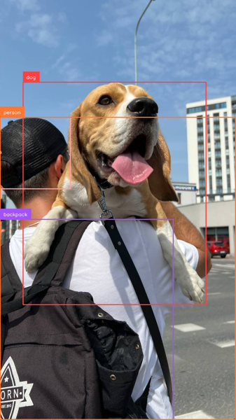
import supervision as sv
from PIL import Image

image = Image.open(EXAMPLE_IMAGE_PATH)
task = "<CAPTION_TO_PHRASE_GROUNDING>"
text = "<CAPTION_TO_PHRASE_GROUNDING> In this image we can see a person wearing a bag and holding a dog. In the background there are buildings, poles and sky with clouds."

inputs = processor(
    text=text,
    images=image,
    return_tensors="pt"
).to(DEVICE)
generated_ids = model.generate(
    input_ids=inputs["input_ids"],
    pixel_values=inputs["pixel_values"],
    max_new_tokens=1024,
    num_beams=3)
generated_text = processor.batch_decode(
    generated_ids, skip_special_tokens=False)[0]
response = processor.post_process_generation(
    generated_text,
    task=task,
    image_size=image.size)
detections = sv.Detections.from_lmm(
    sv.LMM.FLORENCE_2, response, resolution_wh=image.size)

bounding_box_annotator = sv.BoundingBoxAnnotator(
    color_lookup=sv.ColorLookup.INDEX)
label_annotator = sv.LabelAnnotator(
    color_lookup=sv.ColorLookup.INDEX)

image = bounding_box_annotator.annotate(image, detections)
image = label_annotator.annotate(image, detections)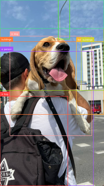
Using LoRA to Optimize Florence-2 Training
The Florence-2 base model we are training has 270 million parameters, which is not much compared to models like Kosmos-2, but still significant if we want to fine-tune our model in Google Colab.
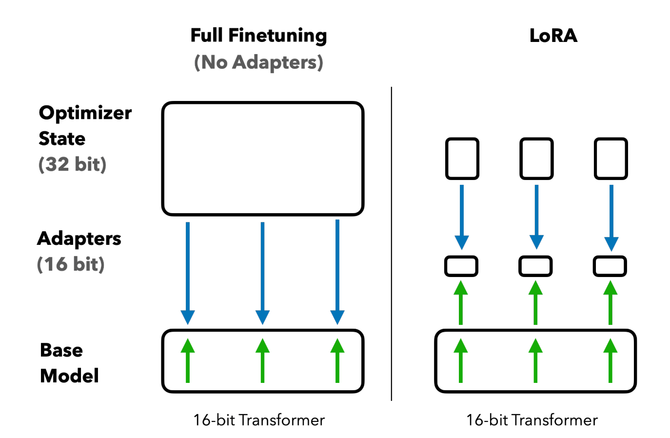
To enable fine-tuning of the full model without freezing specific layers, we will use LoRA, a technique that reduces the number of trainable parameters by adapting only a small subset of the model's weights.
from peft import LoraConfig, get_peft_model

TARGET_MODULES = [
    "q_proj", "o_proj", "k_proj", "v_proj",
    "linear", "Conv2d", "lm_head", "fc2"
]

config = LoraConfig(
    r=8,
    lora_alpha=8,
    target_modules=TARGET_MODULES,
    task_type="CAUSAL_LM",
    lora_dropout=0.05,
    bias="none",
    inference_mode=False,
    use_rslora=True,
    init_lora_weights="gaussian",
    revision=REVISION
)

peft_model = get_peft_model(model, config)
peft_model.print_trainable_parameters()
To use LoRA, we will utilize the perf package. We set r (rank) to 8, lora_alpha (scaling factor) to 8, and lora_dropout to 0.05. The rank controls the dimensionality of the low-rank matrices used in LoRA, while the scaling factor adjusts the magnitude of the LoRA update.
By doing this, we have reduced the number of trainable parameters from approximately 270 million to less than 2 million - a mere 0.7%. This will allow us to use a larger batch size during training.
Fine-tuning Florence-2 Code Overview
Our training loop consists of 3 stages:
Initialization: Before the main loop, we initialize our optimizer, in this case, AdamW, a variant of the Adam optimizer that incorporates weight decay regularization. We also initialize a learning rate scheduler to adjust the learning rate during training.
optimizer = AdamW(model.parameters(), lr=lr)
num_training_steps = epochs * len(train_loader)
lr_scheduler = get_scheduler(
    name="linear",
    optimizer=optimizer,
    num_warmup_steps=0,
    num_training_steps=num_training_steps,
)
Training Loop: Inside the loop iterating over epochs, we have another loop iterating over batches of our training dataset. We perform inference for each batch, and at the end, we trigger backpropagation and calculate the loss.
model.train()
train_loss = 0
for inputs, answers in train_loader:

    input_ids = inputs["input_ids"]
    pixel_values = inputs["pixel_values"]
    labels = processor.tokenizer(
        text=answers,
        return_tensors="pt",
        padding=True,
        return_token_type_ids=False
    ).input_ids.to(DEVICE)

    outputs = model(
        input_ids=input_ids,
        pixel_values=pixel_values,
        labels=labels
    )
    loss = outputs.loss

    loss.backward()
    optimizer.step()
    lr_scheduler.step()
    optimizer.zero_grad()
    train_loss += loss.item()

avg_train_loss = train_loss / len(train_loader)
print(f"Average Training Loss: {avg_train_loss}")
Validation Loop: After each training epoch, we evaluate our model on the validation set. We iterate over batches of the validation set, performing inference for each batch. This time, we do not trigger backpropagation, but only calculate the loss.
model.eval()
val_loss = 0
with torch.no_grad():
    for inputs, answers in val_loader:

        input_ids = inputs["input_ids"]
        pixel_values = inputs["pixel_values"]
        labels = processor.tokenizer(
            text=answers,
            return_tensors="pt",
            padding=True,
            return_token_type_ids=False
        ).input_ids.to(DEVICE)

        outputs = model(
            input_ids=input_ids,
            pixel_values=pixel_values,
            labels=labels
        )
        loss = outputs.loss

        val_loss += loss.item()

    avg_val_loss = val_loss / len(val_loader)
    print(f"Average Validation Loss: {avg_val_loss}")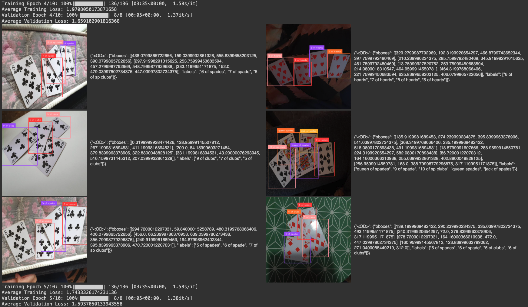
Fine-tuned Florence-2 Model Evaluation
Now that our model is trained, it's time to evaluate its performance. Since we fine-tuned Florence-2 for object detection, we will benchmark our model by calculating the mean Average Precision (mAP) and generating a confusion matrix on the validation subset. We will use the previously installed supervision package for this purpose.
We begin by collecting two lists: target annotations and model predictions. To do this, we loop over our validation dataset and perform inference using our newly trained model. However, to utilize our detections for benchmarking, we need to perform two additional steps:
- Since Florence-2 (unlike traditional detectors like YOLO) does not have a finite set of detectable classes, we need to filter out detections with class names that do not belong to our custom dataset.
- The confusion matrix calculation algorithm requires non-zero confidence values, so we fill them with 1 for each of our detections.
The resulting mAP50:95 value we obtained was 0.52. For comparison, training YOLOv8 version S on the same dataset yielded 0.9. Our training session lasted only 10 epochs and the loss was still decreasing at the time of interruption. It is possible that we could achieve a better mAP value by training the model for a longer duration.
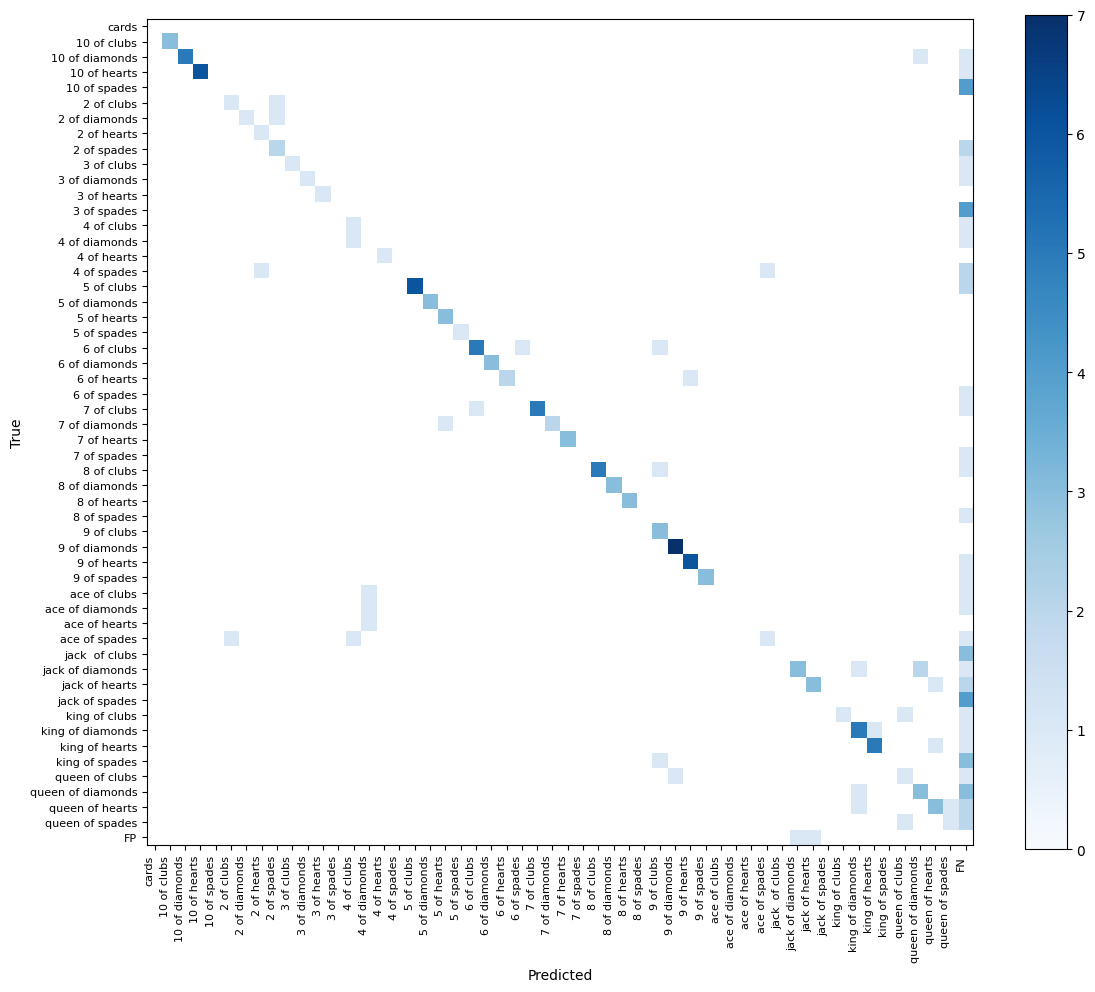
The resulting confusion matrix also looks satisfactory. The vast majority of detections are on the diagonal of our matrix, meaning both the bounding box and the class of our detection are correct.
Generally, we see that if the model detects objects, it does so with the class we expect. Class confusion is rare. Our errors are primarily related to false negatives.
Finally, we verified whether our model could still detect the base classes on which it was pre-trained after completing the training. Models like Florence-2 or PaliGemma may lose some of the capabilities of the pre-trained model as a result of fine-tuning.
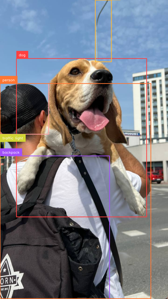
Our test is hardly extensive - it's just one image - but it seems that the model can still detect classes from the COCO dataset.
Deploy Florence-2 Model
Once you have trained your model, you can upload it to Roboflow. You will need to have a dataset in Roboflow to which you can upload your weights. If you do not already have a dataset set up, follow our complete Florence-2 deployment guide where we walk through how to set up a dataset then deploy your model.
If you have a dataset in Roboflow, you can upload your model for deployment using the following code:
import roboflow
rf = Roboflow(api_key="API_KEY")
project = rf.workspace("workspace-id").project("project-id")
version = project.version(VERSION)

version.deploy(model_type="florence-2", model_path="/content/florence2-model")
Above, replace:
API_KEYwith your Roboflow API key.workspace-idandproject-idwith your workspace and project IDs.VERSIONwith your project version.florence-modelwith the saved model directory.
When you run the code above, the model will be uploaded to Roboflow. It will take a few minutes for the model to be processed before it is ready for use.
Step #6: Deploy a Fine-tuned Florence-2 Model
Once your model has been processed, you can download it to any device on which you want to deploy your model. Deployment is supported through Roboflow Inference, our open source computer vision inference server.
Inference can be run as a microservice with Docker, ideal for large deployments where you may need a centralized server on which to run inference, or when you want to run Inference in an isolated container. You can also directly integrate Inference into your project through the Inference Python SDK.
For this guide, we will show how to deploy the model with the Python SDK.
First, install inference:
pip install inference
Then, create a new Python file and add the following code:
import os
from inference import get_model
from PIL import Image
import json

lora_model = get_model("model-id/version-id", api_key="KEY")

image = Image.open("containers.png")
response = lora_model.infer(image)
print(response)
Above, replace:
model-idwith your Roboflow model ID;version-idwith your project version, and;KEYwith your Roboflow API key.
In the code, we load our model, run it on an image, then plot the predictions with the supervision Python package.
When you first run the code, your model weights will be downloaded and cached to your device for subsequent runs. This process may take a few minutes depending on the strength of your internet connection.
Conclusion
Florence-2 is an excellent model with a wide range of supported tasks out of the box. However, if the pre-trained model lacks knowledge about the objects we are looking for, it is possible to fine-tune the model on a custom dataset.
Florence-2 performs worse as a detection model than models created solely for this purpose, such as the latest YOLO models. However, even if it achieves a lower mAP, it has several advantages:
- The fine-tuned model can still detect base classes belonging to the COCO dataset. This can be useful, for example, if we are building an app capable of detecting cars and license plates, we no longer need two separate models. The fine-tuned Florence-2 can detect both classes.
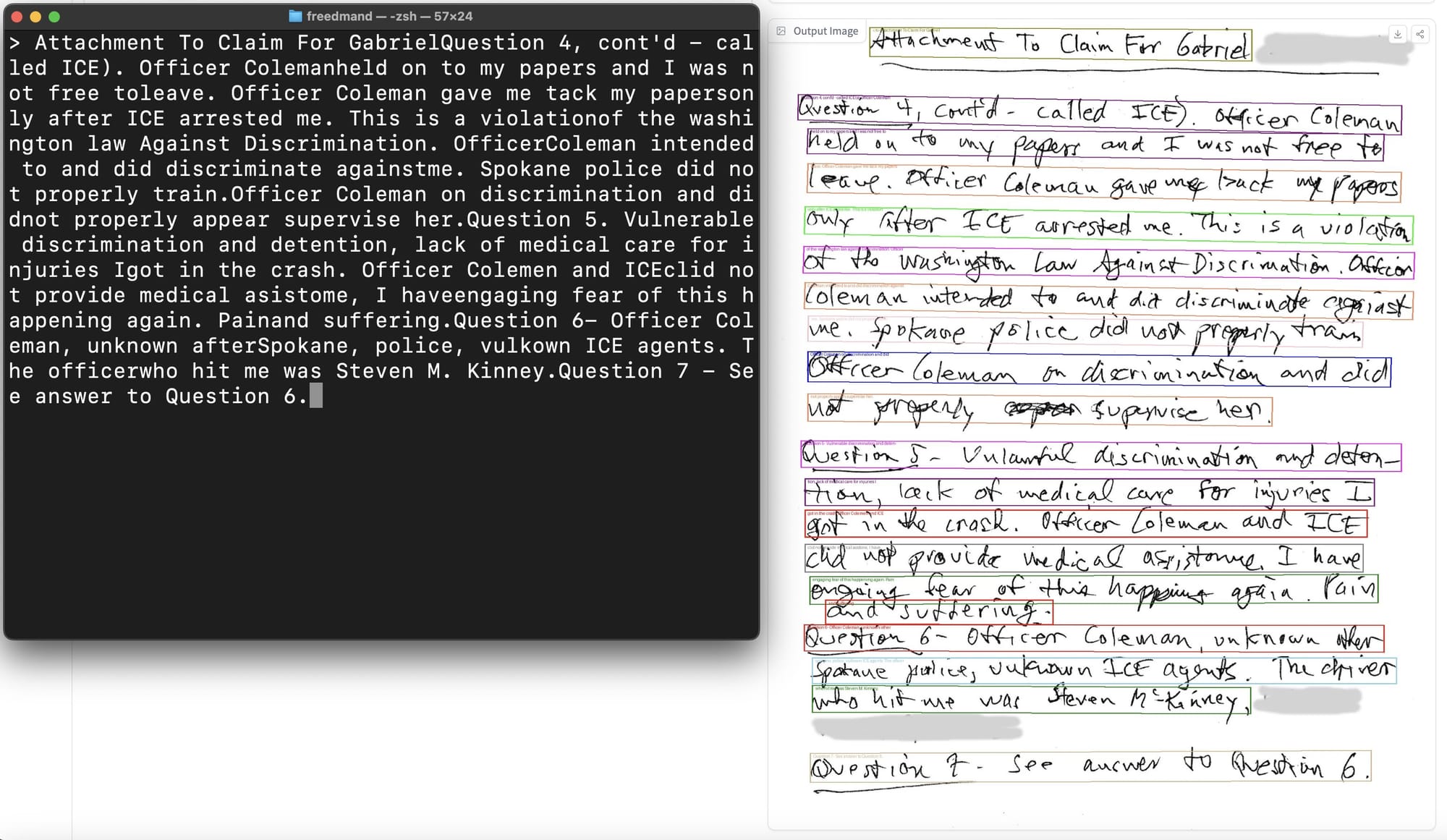
- Florence-2 can perform multiple tasks. Continuing our example with the app that detects cars and license plates, if we additionally want to read the license plate number, we still only need one model. Florence-2 can perform OCR, among other things, and is very good at it.
Additionally, fine-tuning Florence-2 for object detection is less time-intensive than PaliGemma, especially if there is more than one object in the images belonging to our dataset or if our dataset contains many classes.
Cite this Post
Use the following entry to cite this post in your research:
Piotr Skalski. (Jun 25, 2024). How to Fine-tune Florence-2 for Object Detection Tasks. Roboflow Blog: https://blog.roboflow.com/fine-tune-florence-2-object-detection/
