How to Build an Autonomous Defect Detector with Physical AI

Quality inspection on production lines moves fastest when vision systems connect directly to physical hardware. Adding automated defect detection to a manufacturing process catches defects in real time while letting operators focus on higher-level tasks.

Modern computer vision makes physical sorting easy to deploy on standard hardware. Today, ten training photos, a USB webcam, and a desktop robot arm can run the entire detect, decide, pick, and verify loop locally in 0.2 seconds per frame.

How the system works

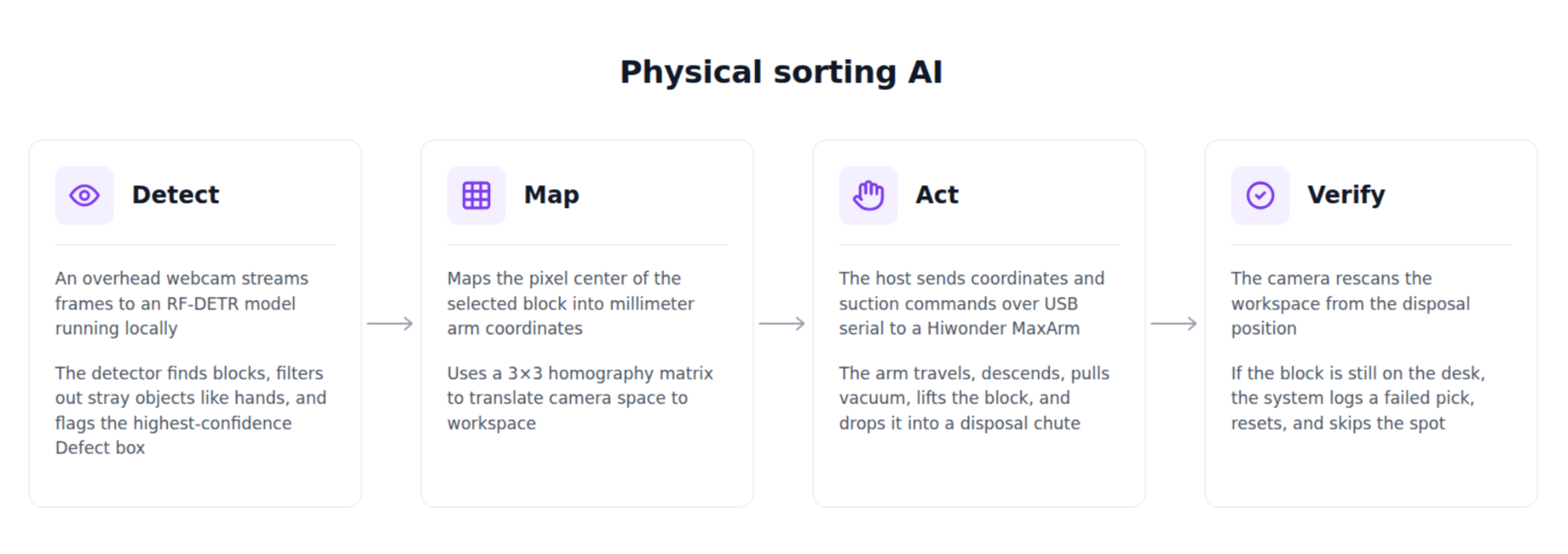
The physical sorting AI works with four steps.

• Detect: An overhead webcam streams frames to an RF-DETR model running locally. The detector finds blocks, filters out stray objects like hands or laptops, and flags the highest-confidence Defect box.
• Map: The system maps the pixel center of the selected block into millimeter arm coordinates using a 3x3 homography matrix.
• Act: The host sends movement coordinates and suction commands over USB serial to a Hiwonder MaxArm. The arm travels, descends, pulls vacuum, lifts the block, and drops it into a disposal chute.
• Verify: The camera rescans the workspace from the disposal position. If the block is still present on the desk, the system logs a failed pick, resets, and skips the spot.

Hardware list

Building a physical board game requires some hardware.

• HiWonder MaxArm: a $200 desktop robot arm driven by an ESP32 controller and equipped with a suction nozzle.

Setting up the repository

You can clone and run the project repository locally:

git clone https://github.com/aarnavshah12/defect-detect-bot && cd defect-detect-bot
uv venv --python 3.12 .venv
uv pip install --python .venv/bin/python opencv-python numpy inference pyserial
echo "ROBOFLOW_API_KEY=your_key_here" > .env

python arm.py --probe              # probes hardware without moving
python arm.py --jog --bootstrap    # you can setup your boundaries and set a home location
python calibrate.py --auto --carry # automated self-calibration routine
python calibrate.py --verify       # test target targeting and nudge offsets
python pick.py --dry-run           # test spatial targeting without hardware motion
python pick.py --once              # execute a single pick cycle
python pick.py                     # run continuous sorting loop

The repository structure separates physical definitions, perception, hardware control, and spatial transformations:

• config.py: Physical dimensions, safety margins, and coordinate bounds. The require() function fails loudly if hardware parameters are missing.
• detect.py: Model loader, Detection dataclasses, spatial filters, and live visualization feeds.
• mapping.py: Homography matrix calculations and coordinate conversions.
• calibrate.py: Self-calibration grid generation, verify nudge routines, and offline error checks.
• arm.py: Serial driver, inverse kinematics wrapper, motion safety bounds, and manual jogging mode.
• pick.py: Main sorting state machine and HUD overlay rendering.
• capture.py: Dataset acquisition tool matching deployment camera parameters.
• tests/: Test suite utilizing mock serial drivers and simulated physics.

Physical calibration parameters on my setup will be much different than yours. Hence, you will need to change and re-calibrate these if you want to replicate.

Annotating data and training RF-DETR

A computer vision model for physical manipulation must be fast, accurate, and resistant to lighting changes on the workbench. 

First, we collected 10 source images using capture.py, a script that forces the webcam to run at the exact resolution and exposure settings used during deployment. Training on your deployment camera prevents lighting and color changes from throwing off the model. Note that 10 source images won’t be enough for real production. Datasets usually include thousands of images to be as accurate as possible. 

Next, we uploaded the images to Roboflow to prepare our dataset for object detection. 

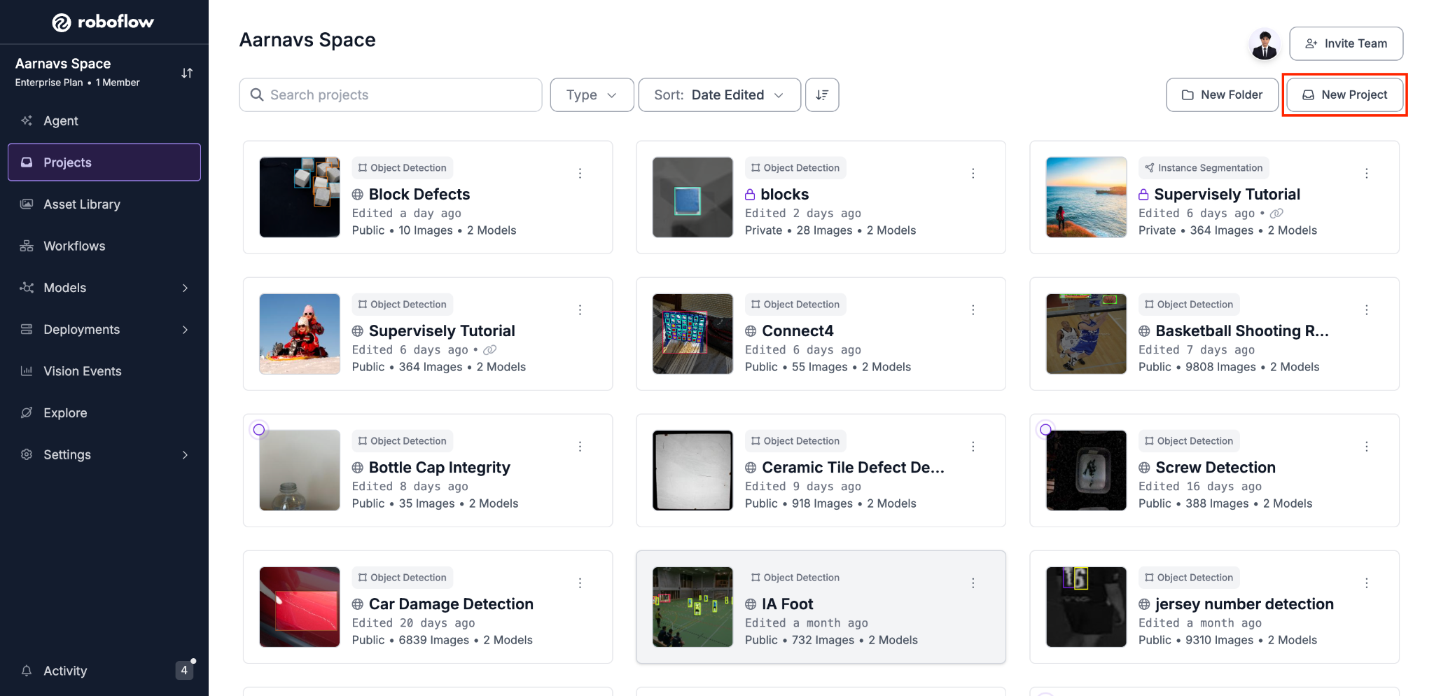
Log into Roboflow first:

Then create a project:

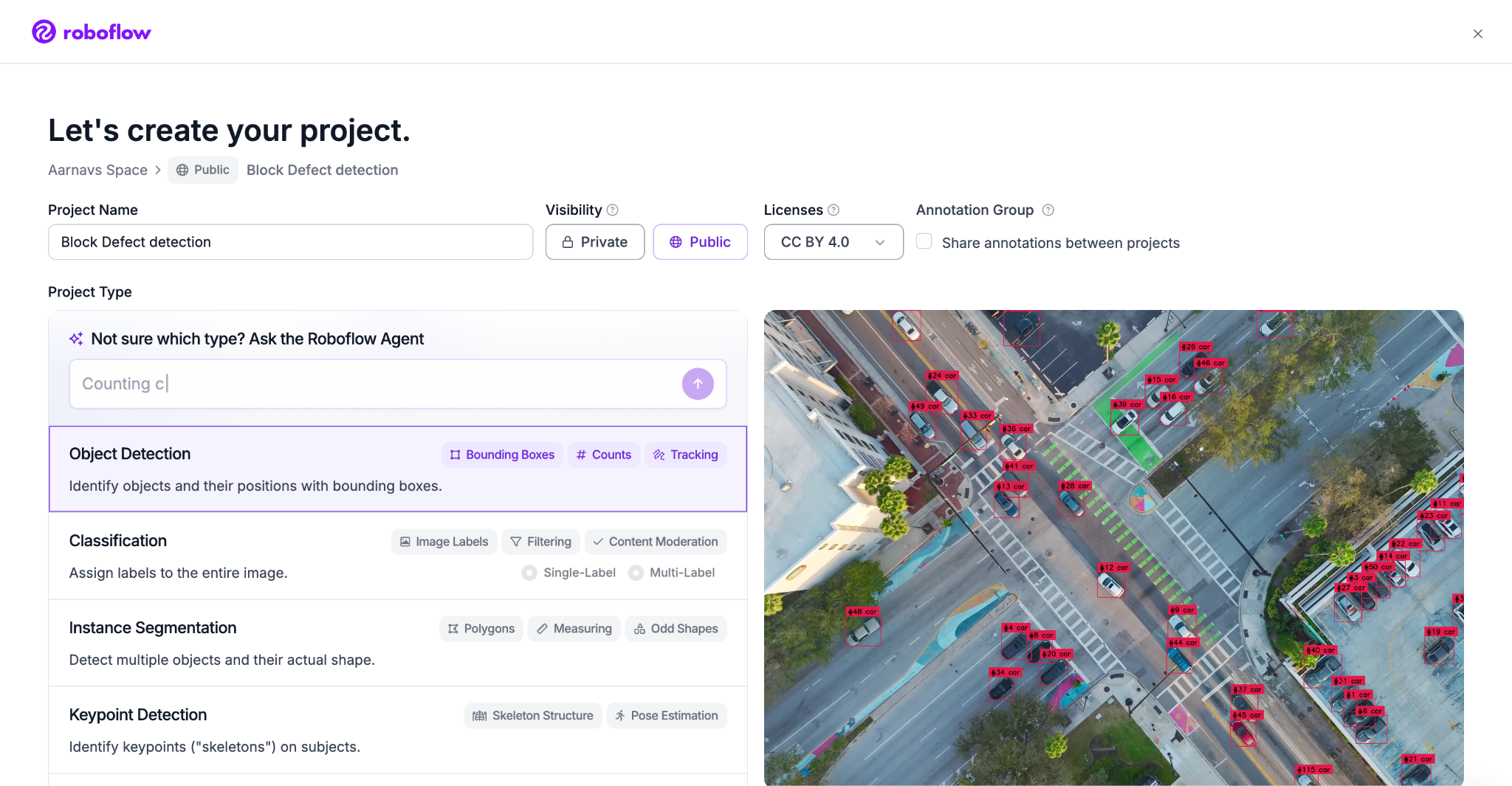
Give it a name and choose object detection:

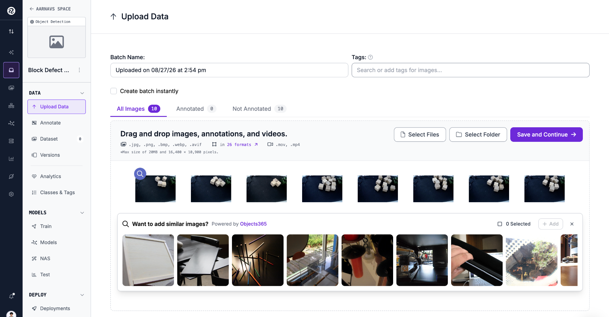
Add your unannotated images in:

Select “Label Manually”:

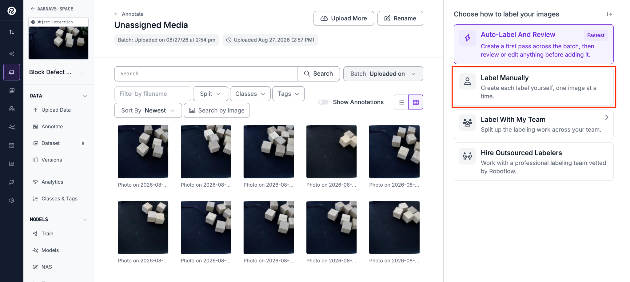
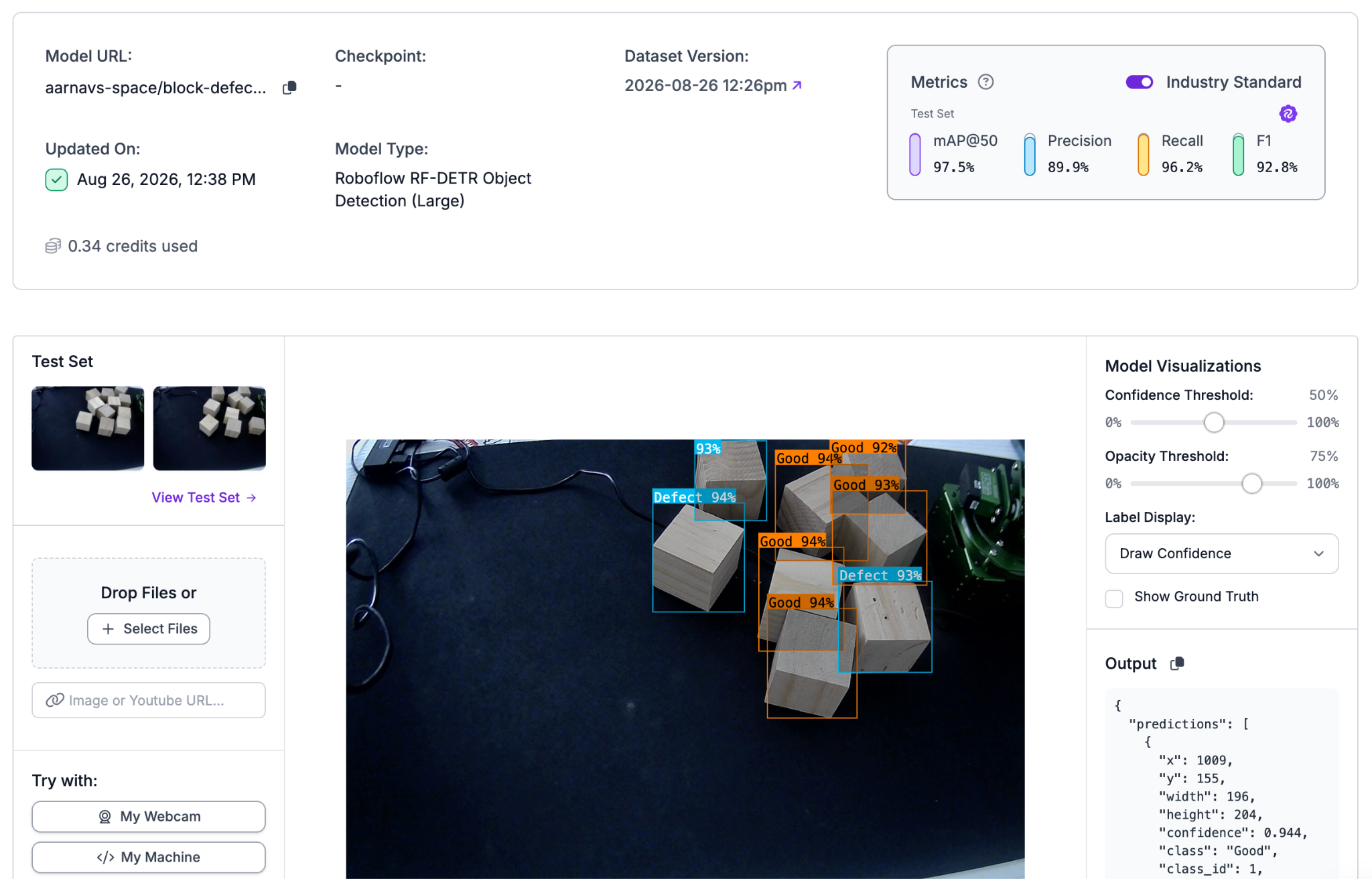
I defined two core classes: “Defect” and “Good”. While I initially considered separating defects into “Hole” and “Scratch”, merging them into a single binary “Defect” class gave our model more training instances per class and simplified the downstream robot logic. This can be altered for larger production datasets, since more images will allow the model to get used to each class, resulting in a more accurate training process.

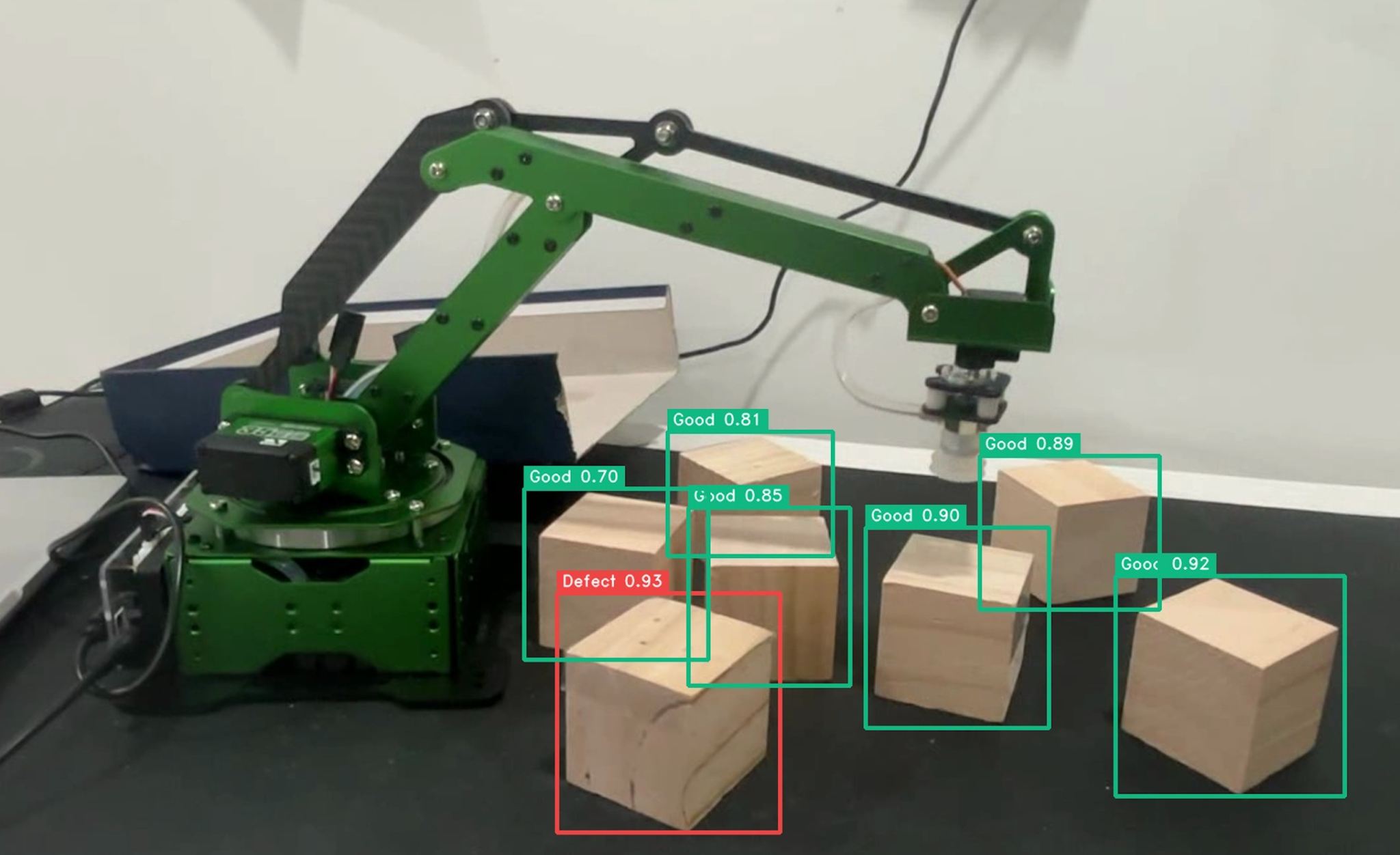
During labeling, I applied three strict annotation guidelines:

1. Draw tight bounding boxes: I labeled bounding boxes flush against the outer edges of each wooden block so the predicted box center matches the true physical center of the object.
2. Label visible features only: If a defect was turned away from the camera, the block was labeled as Good. The model must evaluate only what the camera sees.
3. Include hard negatives: I annotated clean wooden blocks containing dark knots or prominent grain patterns as Good to prevent false positive detections during runtime.

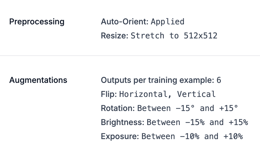
To expand our small dataset, I applied data augmentation inside Roboflow, adding random rotations, brightness shifts, and crop variations. This generated 40 training frames from our 10 original photos.

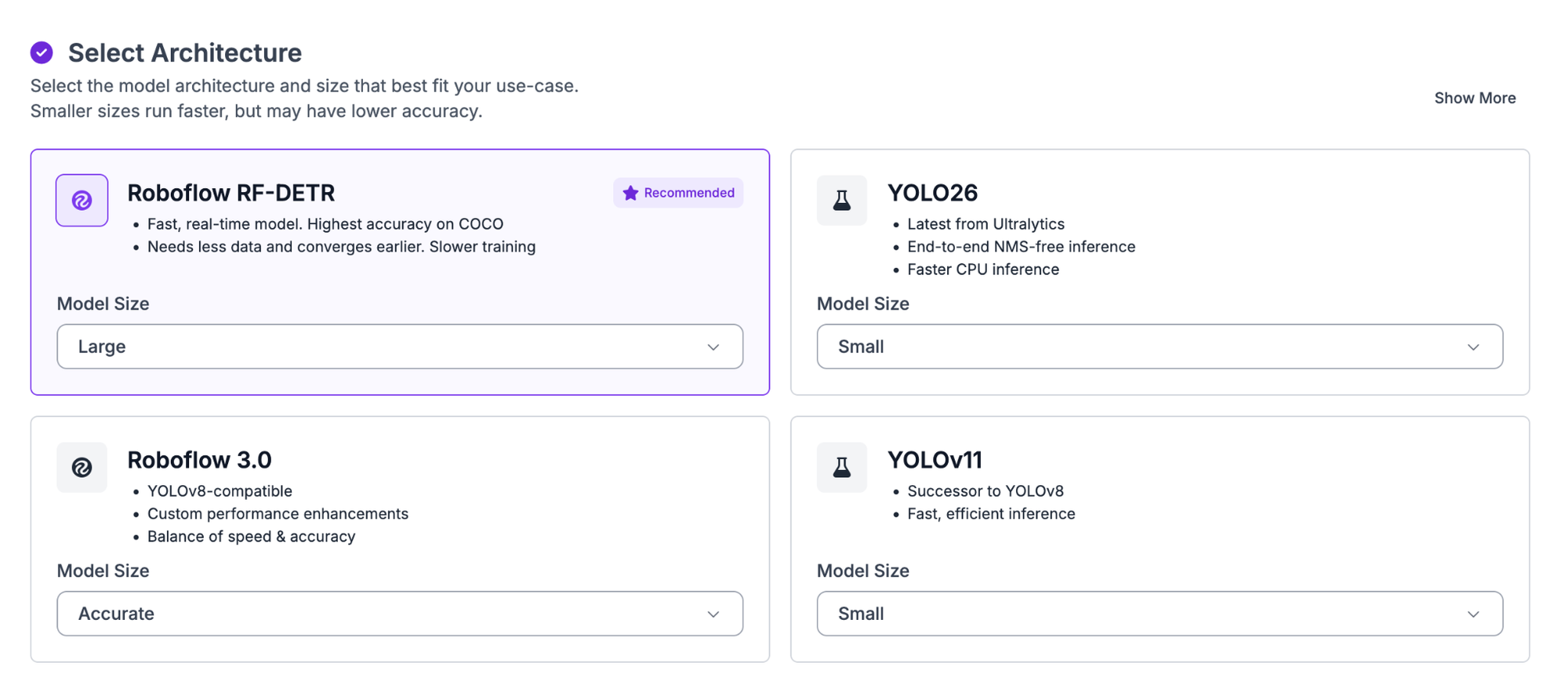
I trained an RF-DETR-large model directly in Roboflow using Custom Training. The model achieved a mAP of 97% on our validation set.

I then exported the trained weights to run locally via CoreML on Apple Silicon, achieving inference latencies of roughly 0.2 seconds per frame.

How to turn pixels into coordinates

To turn detections into action, pixels must map directly to physical coordinates. I solved this using planar camera calibration based on OpenCV's findHomography.

Because the wooden blocks rest on a flat surface, the transformation from camera pixels to physical millimeters is a 3x3 matrix mapping one plane to another. Instead of manually clicking points and typing coordinates, I built an automated self-calibration routine (calibrate.py --auto --carry).

The robot arm picks a single block once, carries it across a 16-point grid, and logs its own commanded positions alongside the detected bounding box centers. This process takes 4 minutes, collects real physical data, and calculates the homography matrix automatically.

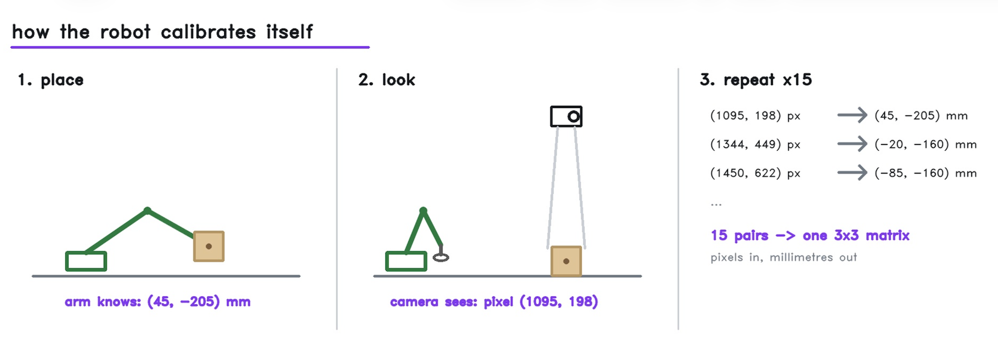
To catch bad calibration points, our script disregards outliers. If someone bumps the table during calibration, the script isolates the pair whose removal reduces global error and names the suspect point. On our final setup, the matrix achieved a mean error of 1.8 mm across the entire pick workspace.

Real-world edge cases

Building physical AI systems reveals edge cases that pure software models never encounter.

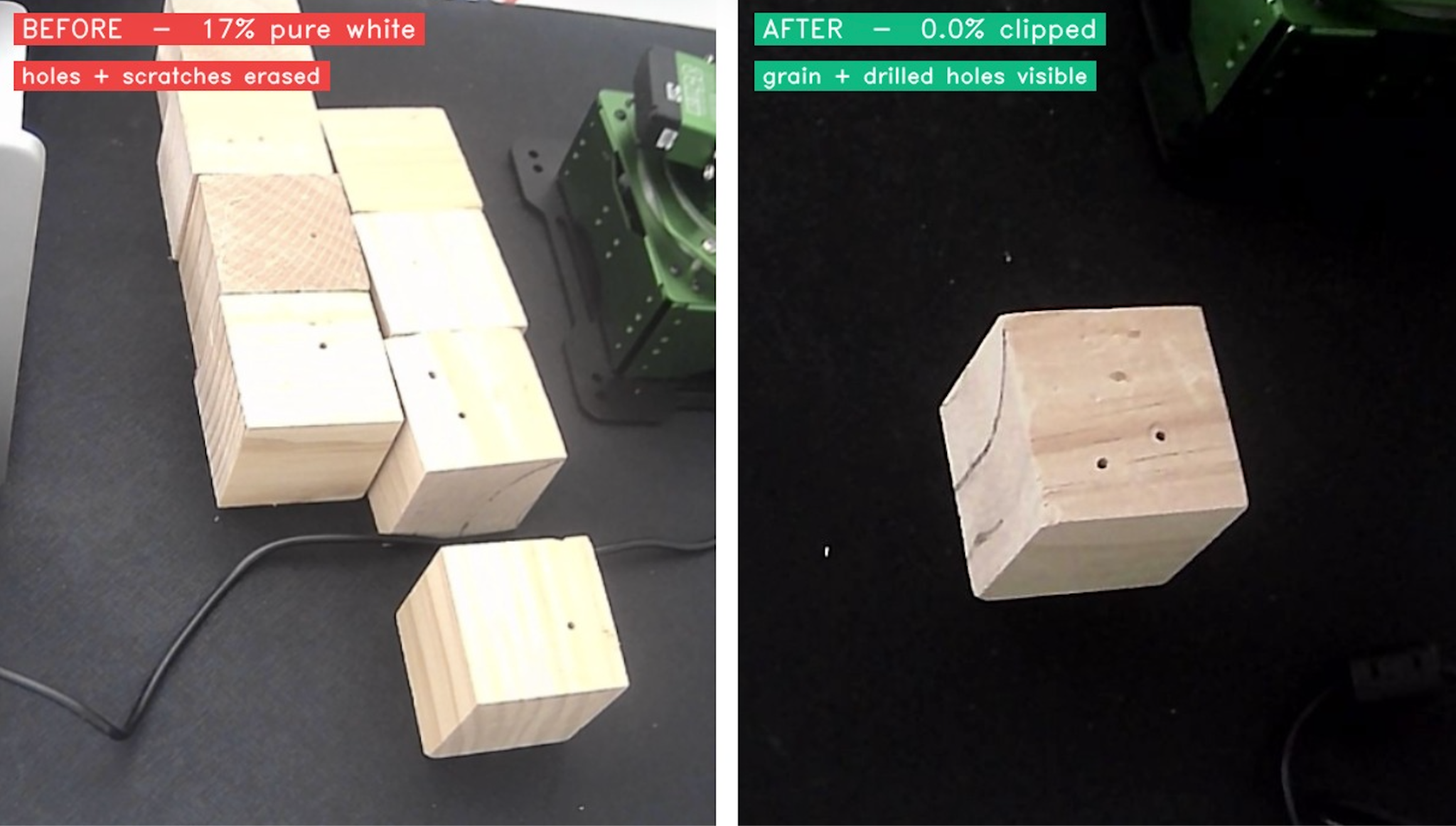
Our first challenge was camera exposure. Under bright overhead lighting, the top faces of the light wood blocks clipped to pure white, erasing surface scratches. Because macOS ignores standard OpenCV exposure commands, we used uvc-util to adjust the camera backlight compensation directly. Setting backlight compensation to 4 forced the auto-exposure algorithm to meter for the bright blocks, dropping image clipping from 14% down to 0.1%.

Our second challenge was suction physics. The most visible defect, a drilled hole in the center of a block, sits directly where the suction cup lands. A hole causes a vacuum leak, causing the block to drop during transport. We resolved this by increasing vacuum build time from 0.5 to 1.0 seconds and adding a slight physical offset to the grip point.

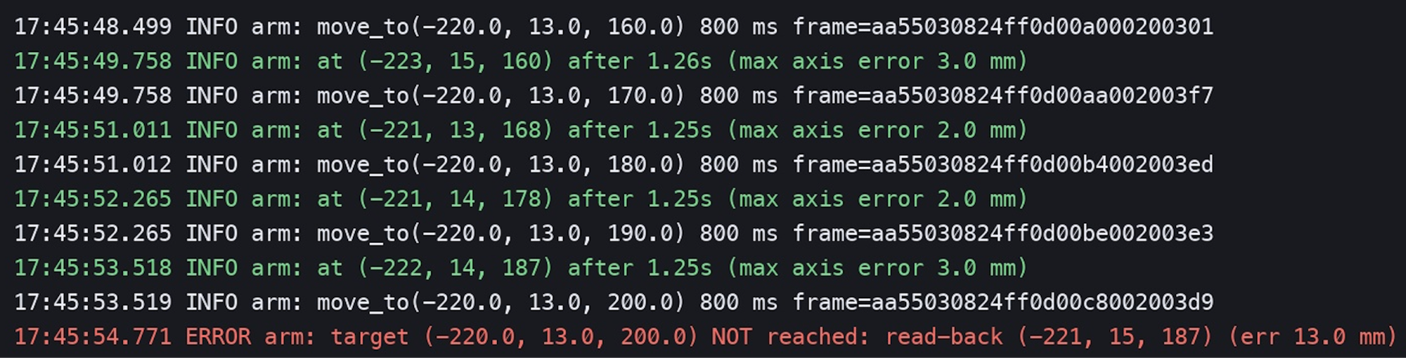
Finally, cheap robot arm controllers do not return move acknowledgments over serial. Unreachable coordinates are dropped without an error message. To solve this, our driver polls the arm's actual joint position after every command. If the reported coordinates differ from the target by more than 10 mm, the system aborts the move, vents the suction valve, and resets.

Scaling beyond wooden blocks

As mentioned before, this defect detection automation can be done with more than wooden blocks. The general sorting architecture (detect, map, act, verify) can apply directly to industrial automation tasks as well:

• Manufacturing quality control: Removing scratched, dented, or misdrilled machined components from production lines.
• Electronics manufacturing: Identifying missing surface-mount components, misaligned chips, or solder bridges on circuit boards.
• Food processing and agriculture: Diverting bruised produce, mouldy items, or foreign material from conveyor belts using air jets or soft grippers.
• Lumber grading: Inspecting wood panels for knots, cracks, and resin pockets to guide automated cutting.
• Textile production: Flagging weave defects, printing misalignments, or stains.
• Pharmaceutical inspection: Rejecting cracked tablets or damaged blister packaging while generating compliance audit logs.

Adapting this system to new industries requires swapping the vision dataset, re-running the 4-minute self-calibration routine, selecting an appropriate end-effector and proper machine. The underlying inference, coordinate mapping, and verification logic remain unchanged.

Build your autonomous defect detection system

You can build a local defect sorting system on your own workbench in five steps.

1. Mount your camera: Clamp a 1080p webcam overhead. Position side lighting to throw shadows across surface defects and lock exposure settings.
2. Train your detector: Collect 100 frames with capture.py, annotate “Defect” and “Good” boxes on Roboflow Annotate, and train an RF-DETR model.
3. Calibrate coordinates: Run arm.py --jog to set your motion boundaries, then run calibrate.py to map pixels to physical millimeter coordinates.
4. Deploy the loop: Run pick.py --dry-run to test spatial targeting, then execute pick.py to start active sorting.
5. Adapt for your application: Swap out the dataset and change the end-effector to match your specific hardware and parts.

Physical AI turns perception into real-world action. Have fun building!

Cite this Post

Use the following entry to cite this post in your research:

Aarnav Shah. (Aug 28, 2026). How to Build an Autonomous Defect Detector with Physical AI. Roboflow Blog: https://blog.roboflow.com/how-to-build-an-autonomous-defect-detector-with-physical-ai/