
RTMDet is a real-time object detector distributed under the Apache 2.0 license that reports 52.8% AP on COCO at over 300 FPS on an NVIDIA 3090, making it a practical choice for commercial projects where restrictive model licenses are a concern. This tutorial walks through training RTMDet on a custom dataset sourced from Roboflow Universe using the OpenMMLab MMDetection and MMYOLO libraries, then evaluating results with Supervision via a confusion matrix and mAP benchmark on a football player detection dataset.
We created a Google Colab notebook that you can run in a separate tab while reading this blog post, allowing you to experiment and explore the concepts discussed in real time. Let’s dive in!
Introduction
Looking for a state-of-the-art object detector that you can use in an enterprise project is difficult. Most popular models come with a license that forces you to open-source your entire project. Today I'm going to show you how to train an RTMDet - a model that is fast and accurate enough to compete with top models, but which - due to its open license - you can use anywhere.
What is RTMDet?
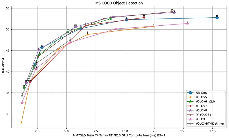
RTMDet is an efficient real-time object detector, with self-reported metrics outperforming the YOLO series. It achieves 52.8% AP on COCO with 300+ FPS on an NVIDIA 3090 GPU, making it one of the fastest and most accurate object detectors available as of writing this post.
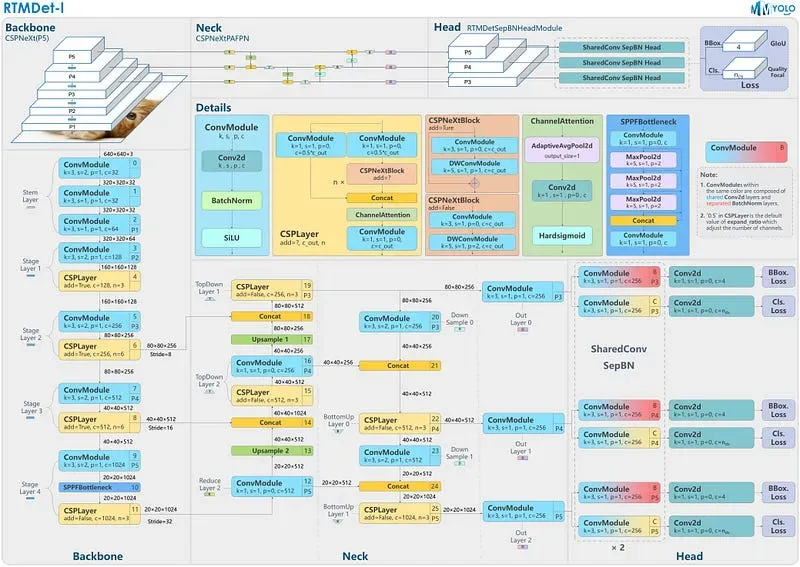
RTMDet utilizes an architecture with compatible capacities in both the backbone and neck, constructed using a basic building block comprising large-kernel depth-wise convolutions. This design enhances the model’s ability to capture global context while maintaining fast inference speed.
Importantly, RTMDet is distributed through MMDetection and MMYOLO packages under the Apache-2.0 license. Accuracy, speed, ease of deployment, and a permissive license make RTMDet an ideal model for enterprise users building commercial applications.
What is OpenMMLab?
OpenMMLab covers a wide range of research topics of computer vision, such as classification, detection, segmentation, and super-resolution. A distinctive feature of this framework is that it is divided into many libraries of limited scope.
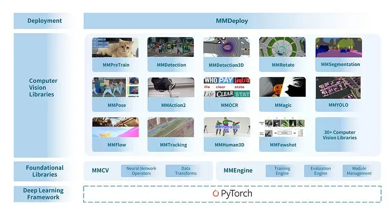
OpenMMLab has released 30+ vision libraries, has implemented 300+ algorithms, and contains 2000+ pre-trained models. All the libraries have accumulated tens of thousands of stars on GitHub.
This tutorial will use four libraries from the OpenMMLab ecosystem:
- MMEngine — Foundational library for training deep learning models.
- MMCV — Foundational library for computer vision.
- MMDetection — Detection toolbox and benchmark.
- MMYOLO — YOLO series toolbox and benchmark. It offers state-of-the-art object detection models such as YOLOv7, YOLOv8, PP-YOLOE, and RTMDet.
OpenMMLab Libraries Installation
Let’s start by setting up the Python environment. MMYOLO relies on PyTorch, MMCV, MMEngine, and MMDetection.
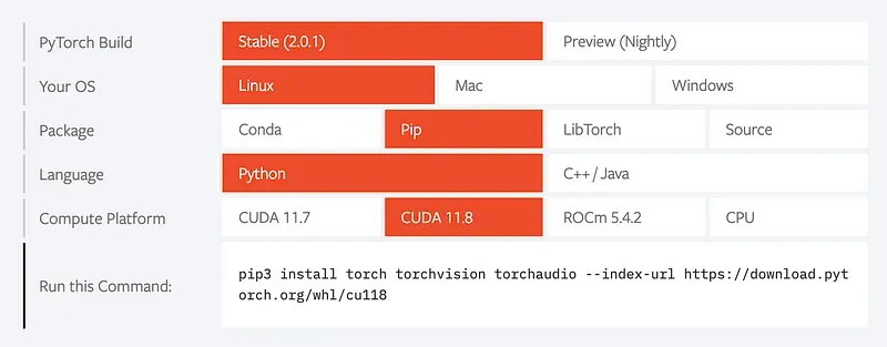
When installing PyTorch, make sure to choose a version that is suitable for your hardware and operating system. A tool on the official site will help you compose the right installation command.
OpenMMLab has its own package manager — MIM. Take a peek below for quick installation steps. Please refer to the Install Guide for more detailed instructions.
cd {HOME}
pip install -U -q openmim
mim install -q "mmengine>=0.6.0"
mim install -q "mmcv>=2.0.0rc4,<2.1.0"
mim install -q "mmdet>=3.0.0rc6,<3.1.0"
git clone https://github.com/open-mmlab/mmyolo.git
cd {HOME}/mmyolo
mim install -v -e .
Finally, let’s install two more Python libraries. roboflow— which we will use to download the dataset from Roboflow Universe. supervision— which will provide us with utilities to visualize detections, load datasets, and benchmark the model.
pip install -q roboflow supervisionInference with Pre-trained RTMDet COCO model
RTMDet architecture comes in five different sizes: RTMDet-t, RTMDet-s, RTMDet-m, RTMDet-l, and RTMDet-x. Throughout this tutorial, we will use one of the larger versions — RTMDet-l . Remember that depending on your use case, your decision may differ. Take a peek at Figure 1. visualizing the speed-accuracy tradeoff.
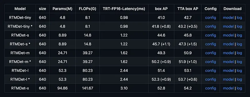
Once you have chosen the model size you want to use, it is time to download the appropriate configuration file and pre-trained weights. You can find the necessary links in the table in the MMYOLO repository’s README. Download the proper files to your hard drive and save them under the CONFIG_PATH and WEIGHTS_PATH paths.
import torch

from mmdet.apis import init_detector

DEVICE = torch.device('cuda:0' if torch.cuda.is_available() else 'cpu')
CONFIG_PATH = '...'
WEIGHTS_PATH = '...'

model = init_detector(CONFIG_PATH, WEIGHTS_PATH, device=DEVICE)
Now we are ready to initialize the model. All we have to do is call the init_detector function available in MMDetection API, providing it with CONFIG_PATH, WEIGHTS_PATH, and DEVICE as arguments. The value of DEVICE will vary depending on your hardware and the version of PyTorch you have installed.
import cv2
import supervision as sv

from mmdet.apis import inference_detector

IMAGE_PATH = '...'
image = cv2.imread(IMAGE_PATH)

result = inference_detector(model, image)
detections = sv.Detections.from_mmdetection(result)
box_annotator = sv.BoxAnnotator()
annotated_image = box_annotator.annotate(image.copy(), detections)
We can now use the model to infer any image or video. We visualize the results using BoxAnnotator available in the supervision library.
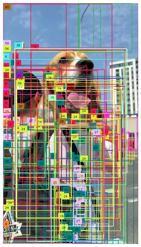
By default, the result of MMDetection inference looks chaotic. The model returns several hundred proposed bounding boxes. We must filter out detections based on their confidence and use NMS to combine double-detections. We can do this by adding one line of supervision code. I encourage you to read more about the advanced detection filtering mechanisms available in supervision.
import cv2
import supervision as sv

from mmdet.apis import inference_detector

IMAGE_PATH = '...'
image = cv2.imread(IMAGE_PATH)

result = inference_detector(model, image)
detections = sv.Detections.from_mmdetection(result)
detections = detections[detections.confidence > 0.3].with_nms()
box_annotator = sv.BoxAnnotator()
annotated_image = box_annotator.annotate(image.copy(), detections)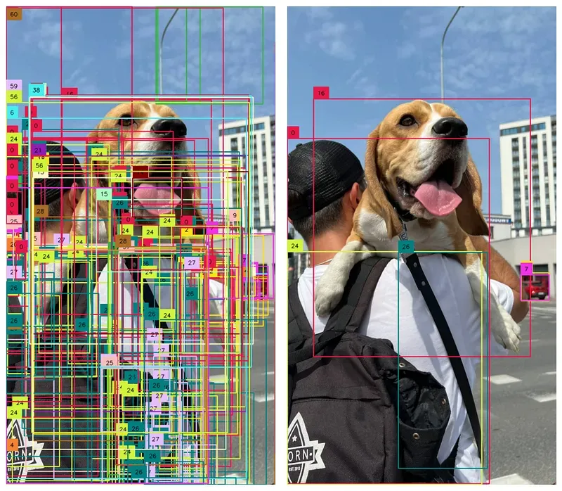
Downloading a Dataset from Roboflow Universe
To train a model with the MMDetection framework, we need a dataset in COCO format. In this tutorial, I will use the football-player-detection dataset. Feel free to replace it with your dataset or another dataset from Roboflow Universe.

If you use a dataset from Roboflow Universe, export it in COCO-MMDetection format. This ensures smooth integration in the training process.
One more thing. If you want to use your dataset but it is not in COCO format, no problem. You can use the supervision to convert it from PASCAL VOC or YOLO to COCO.
import roboflow

roboflow.login()
rf = roboflow.Roboflow()

WORKSPACE_NAME = "roboflow-jvuqo"
PROJECT_NAME = "football-players-detection-3zvbc"
PROJECT_VERSION = 2

project = rf.workspace(WORKSPACE_NAME).project(PROJECT_NAME)
dataset = project.version(PROJECT_VERSION).download("coco-mmdetection")With Auto Label, you can use foundation models like Grounding DINO and Segment Anything to automatically label images in your dataset. Refer to our Auto Label launch post for more information about how Auto Label works, and how you can use it with your project.
Preparing Custom MMDetection Configuration File
Crafting a custom configuration file is the most overwhelming aspect of the MMDetection framework.
The best strategy is to copy the raw configuration file of the model you want to train and make changes. In my case, the original configuration file for the RTMDet-l model needed several extra important elements.
Let’s start by providing information on the dataset. Paths to the image directory and annotation JSON for train and validation subsets, as well as the list and number of class names.
data_root = '.data/football-players-detection-2/'

train_ann_file = 'train/_annotations.coco.json'
train_data_prefix = 'train/'

val_ann_file = 'valid/_annotations.coco.json'
val_data_prefix = 'valid/'

class_name = ('ball', 'goalkeeper', 'player', 'referee')
num_classes = 4
As usual, we must define typical training parameters: batch size, learning rate, input image size, and epoch count.
train_batch_size_per_gpu = 8
base_lr = 0.004
max_epochs = 50
img_scale = (640, 640)
Finally, it is a good idea to define integration with Tensor Board or Weights & Biases.
_base_.visualizer.vis_backends = [
dict(type='LocalVisBackend'),
dict(type='TensorboardVisBackend'),]
Train RTMDet and Analyze the Metrics
Once we have a complete configuration file, most of the work is already behind us. All we have to do is run the train.py script and be patient. The training time depends on the chosen model architecture, the size of the dataset, and the hardware you have.
cd {HOME}/mmyolo
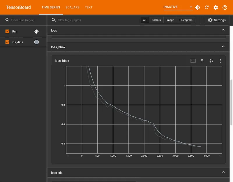
python tools/train.py configs/rtmdet/custom.pyWhen the training ends, all artifacts will be saved in the mmyolo/work_dirs directory. There we will find our model's weights and configuration file and, if we have configured integration with Tensor Board, the logs that we can visualize. All we need to do is update the tensorboard argument —-logdir so that it leads to the work_dirs associated with the training job.
Evaluating the RTMDet Model with Supervision
It is good practice to evaluate the model after the training. It is important not to benchmark the model on images we previously used during training. The goal is to test how well the model will handle images it has not seen before.
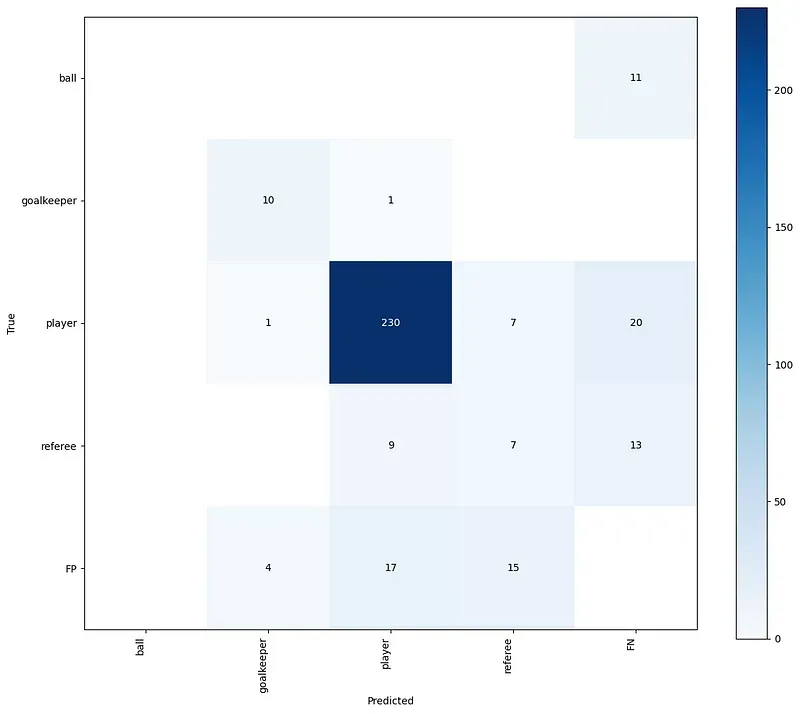
The confusion matrix visualizes model performance by comparing its predicted classifications to actual ground truth values, highlighting true positives, false positives, true negatives, and false negatives. To do this, we will use the previously installed supervision pip package.
We load our dataset from the hard drive, define an inference callback (containing our trained model), and are ready to go.
IMAGES_DIRECTORY = f"{dataset.location}/test"
ANNOTATIONS_PATH = f"{dataset.location}/test/_annotations.coco.json"

ds = sv.DetectionDataset.from_coco(
	images_directory_path=IMAGES_DIRECTORY,
	annotations_path=ANNOTATIONS_PATH,
)

def callback(image: np.ndarray) -> sv.Detections:
	result = inference_detector(model, image)
	detections = sv.Detections.from_mmdetection(result)
	detections = detections[detections.confidence > 0.3]
	return detections.with_nms(threshold=0.7)

confusion_matrix = sv.ConfusionMatrix.benchmark(
	dataset = ds,
	callback = callback
)
confusion_matrix.plat()
Just one look at the confusion matrix gives us a lot of information about our dataset and the model trained with it. Our data set is highly unbalanced — most annotations represent the player class. In contrast, our model does well with detecting goalkeepers and players, poorly with referees, and badly with the ball.
Mean average precision (mAP) is another metric often used to benchmark object detection models. It lets you describe the model's accuracy using a single number between 0 and 1.
mean_average_precision = sv.MeanAveragePrecision.benchmark(
	dataset = ds,
	callback = callback
)
mean_average_precision.map50_95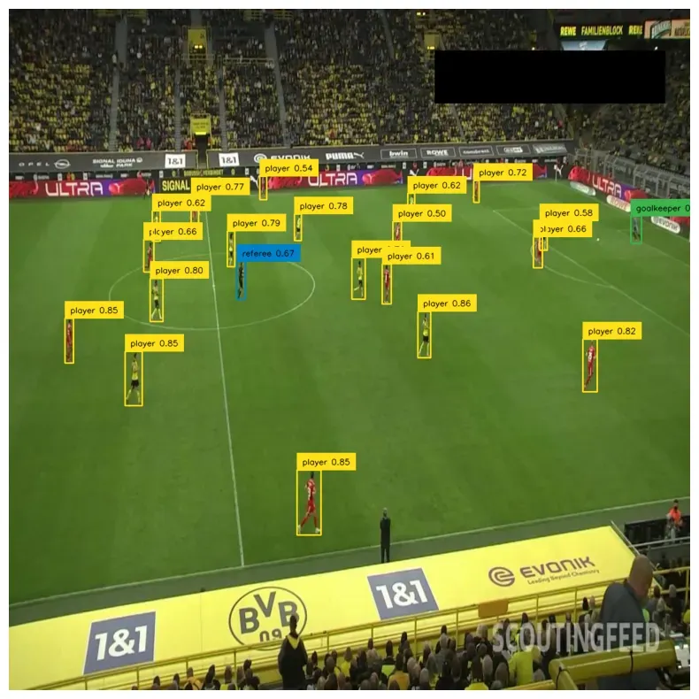
Conclusion
We encourage you to use the Google Colab notebook provided, delve deeper into the configurations, and experiment with different model architectures from the OpenMMLab ecosystem.
Cite this Post
Use the following entry to cite this post in your research:
Piotr Skalski. (Aug 9, 2023). How to Train RTMDet on a Custom Dataset. Roboflow Blog: https://blog.roboflow.com/how-to-train-rtmdet-on-a-custom-dataset/