

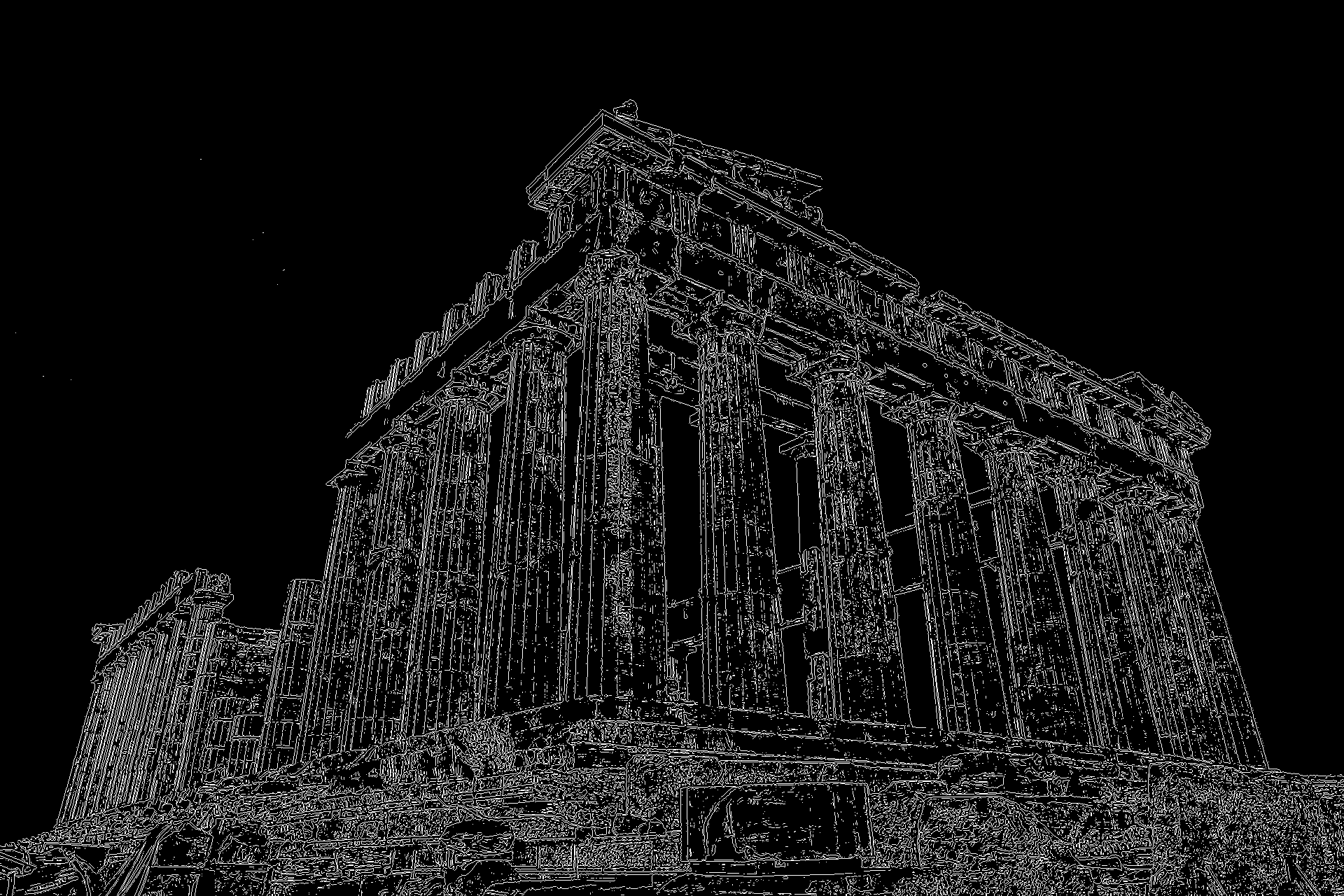
Laplacian Edge Detection is a computer vision technique used to identify the boundaries of objects and regions in an image or video frame. It applies a Laplacian kernel to detect regions where the rate of image intensity change varies rapidly, which can indicate the presence of an edge.
Edges play an important role in computer vision by helping identify the boundaries of objects, shapes, and regions within an image. Detecting these boundaries can simplify an image while preserving important visual information, making it easier to analyze and process before applying more advanced computer vision techniques.
Several edge detection techniques can be used for this purpose, including Laplacian Edge Detection, Canny Edge Detection, and Sobel Edge Detection. Among these techniques, Laplacian Edge Detection detects edges by identifying regions where the rate of intensity change varies rapidly, indicating potential edges.
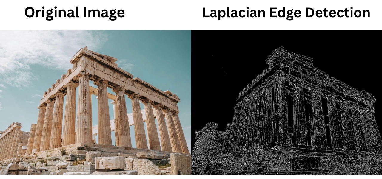
In this guide, you’ll learn what Laplacian Edge Detection is, what first-order and second-order derivatives are in image processing, how Laplacian Edge Detection works, how it differs from Sobel and Canny Edge Detection, and how to implement it using Roboflow Workflows.
What Is Laplacian Edge Detection?
Laplacian Edge Detection is a computer vision technique used to detect edges by measuring how quickly the rate of pixel intensity changes varies. Sobel Edge Detection measures the rate at which pixel intensity changes, using first-order derivatives. In contrast, Laplacian Edge Detection measures how quickly this rate of change itself varies, using second-order derivatives.
Sobel Edge Detection uses first-order derivatives to calculate the rate of change in pixel intensity separately in the horizontal and vertical directions. A large change in intensity in either direction indicates a potential edge.
The Laplacian uses second-order derivatives to measure how quickly the rate of intensity change varies in the horizontal and vertical directions. It combines these changes into a single response. Rapid changes in the rate of intensity change produce a strong Laplacian response, which can indicate the presence of an edge.
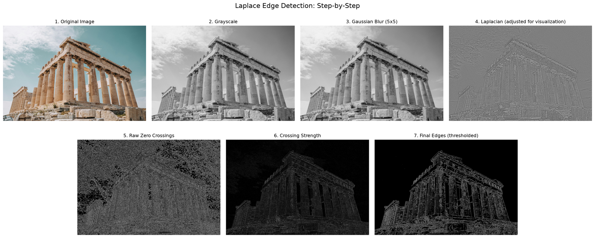
Laplacian Edge Detection generally involves the following steps:
- Convert the image to grayscale.
- Apply a Gaussian blur to reduce noise and small intensity variations.
- Apply a Laplacian kernel to calculate the second-order derivative of the image.
- Detect zero crossings where the Laplacian response changes from positive to negative or negative to positive. These locations indicate potential edges.
- Apply a threshold to remove weak zero-crossing responses caused by noise or insignificant intensity variations, producing a binary edge image.
Advantages of Laplacian Edge Detection
- Isotropic (Rotation Invariant): Detects edges in all directions, including horizontal, vertical, and diagonal, using a single kernel convolution. Unlike Sobel, it does not require separate convolutions for different directions.
- Precise Edge Localization: Zero-crossing detection locates the exact center of an edge transition, yielding thin, single-pixel-wide contours rather than broad gradient bands.
- High Sensitivity to Fine Detail: Accurately captures high-frequency visual components and rapid intensity changes that first-order derivatives might smooth over.
Disadvantages of Laplacian Edge Detection
- High Sensitivity to Noise: Second-order derivatives heavily magnify high-frequency spatial noise. Pre-filtering with a Gaussian blur (forming a Laplacian of Gaussian, or LoG filter) is almost always needed.
- No Directional Information: Shows where an edge exists and how sharp it is, but does not indicate the edge's orientation or angle.
- Double-Edge Effect: Creates two responses (a positive and a negative) on opposite sides of a thick boundary, which can result in unwanted double-line contours.
- False Edges: Minor texture variations or light flickers can trigger false edges, creating faint, unintended outlines in textured areas unless strict thresholding is used.
What is First-Order Derivative and Second-Order Derivative in Image Processing?
To understand how Laplacian Edge Detection works, it helps to first understand what first-order and second-order derivatives measure in an image.
First-Order Derivative
A first order derivative measures the rate of change of pixel intensity, or how quickly the intensity changes as we move through the image.
This is important for edge detection because an edge usually occurs at a location where the pixel intensity changes rapidly. Therefore, a large first order derivative indicates a strong intensity transition and can be used to identify potential edges.
For an image intensity function I(x, y), the first order derivatives can be represented using the gradient operator. The gradient at each pixel is defined as:

The gradient describes how the image intensity changes in the horizontal (x) and vertical (y) directions.
Since the gradient contains two components, we can calculate its magnitude to determine the overall strength of the intensity change at each pixel:

The magnitude of the gradient gives a single value representing how strongly the intensity changes, regardless of the direction of the change. A large gradient magnitude means that the intensity changes rapidly around that pixel, making it a likely location of an edge. Conversely, a small gradient magnitude indicates that the intensity is changing slowly, which is more typical of a relatively uniform region.
Sobel Edge Detection approximates the first order derivatives in the horizontal and vertical directions and uses them to estimate the gradient magnitude. Pixels with sufficiently large gradient magnitudes are then identified as potential edges.
Second-Order Derivative
A second-order derivative measures how quickly the first-order rate of change itself changes. In image processing, it describes how the rate of change of image intensity varies as we move through the image.
The second-order derivative can be represented using the Laplacian operator. The Laplacian measures how much the rate of change of intensity at a pixel differs from the rate of change of intensity in its surrounding pixels.
For a image, the Laplacian is given by:

The first term represents the second-order change in the horizontal direction (x), while the second term represents the second-order change in the vertical direction (y). The Laplacian combines these two values into a single value at each pixel. This gives the overall second-order change in intensity without focusing on a particular direction.
The Laplacian produces a strong response where the rate of change of image intensity changes rapidly. An edge is often found near a point where the Laplacian changes sign, such as from positive to negative or negative to positive.
How Does Laplacian Edge Detection Work?
Laplacian edge detection typically involves converting the image to grayscale, smoothing it with a Gaussian blur, applying the Laplacian operator, and detecting zero crossings in the resulting response. A threshold can then be used to remove weak zero crossings caused by noise or insignificant intensity variations.
Step 1: Convert the Image to Grayscale
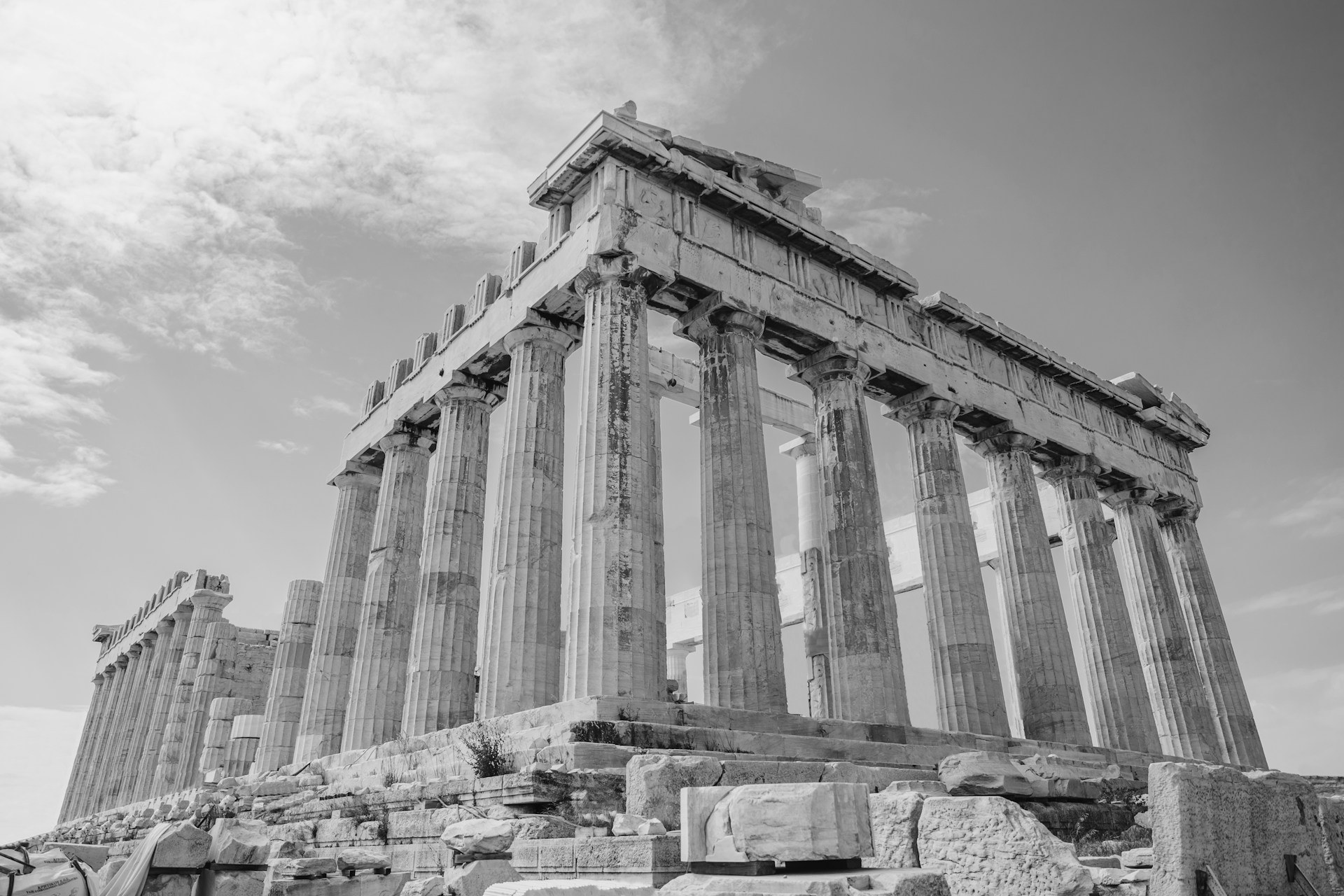
The input image is first converted to grayscale. This reduces the image to a single intensity value for each pixel, making it easier to calculate changes in brightness.
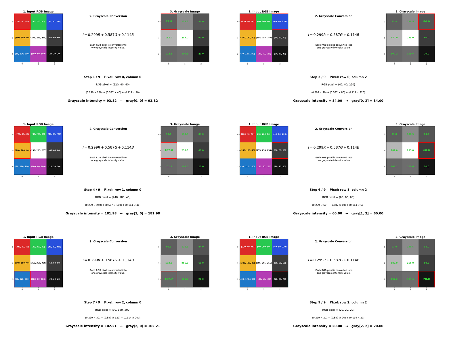
A common grayscale conversion combines the red, green, and blue intensity values of each pixel using the following weighted formula:

Here, (R), (G), and (B) represent the red, green, and blue intensity values of each pixel, while (I) represents the resulting grayscale intensity.
The visualization below shows how a RGB color image is converted into a grayscale image using the weighted formula:
The example below shows the conversion of a real-world (RGB) image to a single-channel, grayscale image.
Step 2: Apply Gaussian Blur
Second-order derivatives are sensitive to small intensity variations, the Laplacian can also respond strongly to noise. A Gaussian blur is therefore commonly applied before the Laplacian operation to reduce noise and unwanted intensity variations.
The grayscale image is smoothed using a Gaussian blur to reduce noise and small variations in pixel intensity. Small changes caused by noise can produce strong Laplacian responses and result in unwanted edges.
Gaussian blurring is performed by convolving the image with a Gaussian kernel. Convolution is an operation that applies a kernel to an image by placing it over a local region, multiplying the kernel values by the corresponding pixel values, and summing the results. The resulting sum replaces the value of the center pixel of that region. The kernel is then moved to the next pixel, and the process is repeated across the image. For example, a Gaussian kernel can be represented as:

The visualization below shows how the Gaussian kernel moves across the image and calculates the new pixel values at each position.
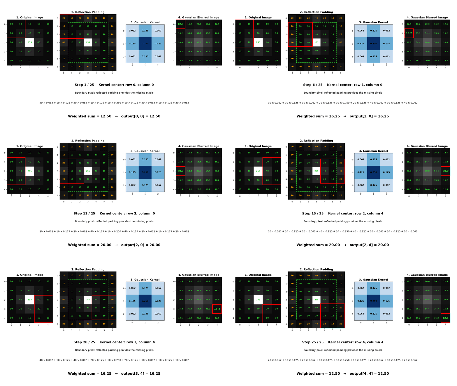
The Gaussian kernel gives higher weights to pixels near its center and lower weights to pixels farther away. As a result, each new pixel value is a weighted average of the surrounding pixels. This reduces small intensity variations, producing a smoother image with less high-frequency noise.
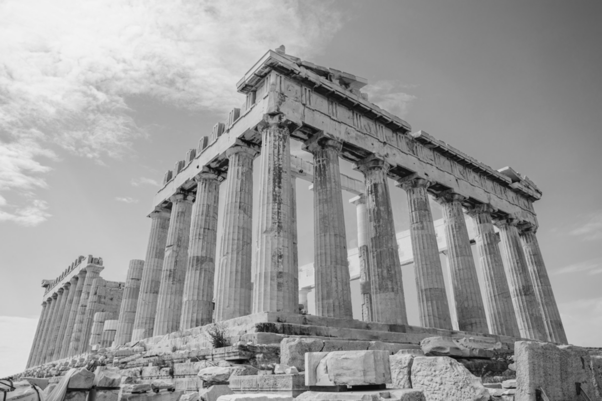
The example below shows the grayscale image after light Gaussian smoothing with a 3×3 kernel. The image is not heavily blurred, but fine noise is suppressed while the main structures and edges remain sharp enough to be detected.
Step 3: Apply the Laplacian Kernel
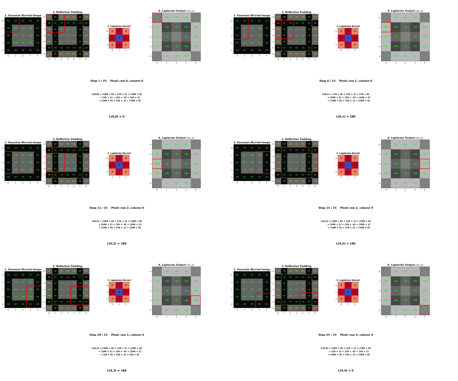
The blurred grayscale image is then convolved with a Laplacian kernel to approximate second-order change in pixel intensity. A commonly used 3×3 Laplacian kernel is:

The convolution of the image with the Laplacian kernel combines the second-order derivatives in the horizontal and vertical directions to produce a single Laplacian value, L(x, y), for each pixel:

Unlike Sobel Edge Detection, which calculates the first-order intensity changes separately in the horizontal and vertical directions by convolving the image with two different kernels and then combining the results into a gradient magnitude, the Laplacian combines the second-order changes from both directions into a single response by convolving the image with a single Laplacian kernel.
The visualization below shows how the Laplacian kernel moves across the image and calculates the new pixel values at each position.
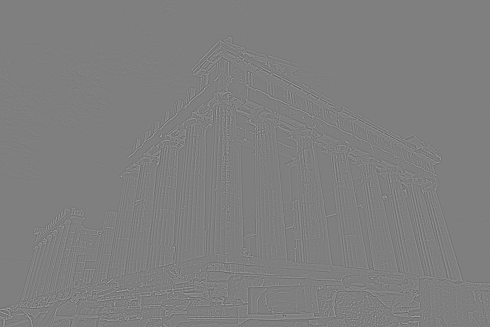
The example below shows the Laplacian values represented as a zero-centered grayscale image.
Step 4: Detect Zero Crossings
A zero crossing occurs when the Laplacian value changes from positive to negative or from negative to positive between neighboring pixels. These sign changes can indicate the location of an edge in the image.
For example, if two neighboring pixels have Laplacian values of +20 and -15, the response changes from positive to negative, indicating a zero crossing between them.
Mathematically, a zero crossing between two neighboring pixels can be identified when their Laplacian values have opposite signs:

Here, the multiplication of the two Laplacian values gives a negative result because they have opposite signs. This indicates a zero crossing between the two neighboring pixels:

Once a zero crossing is detected between two neighboring pixels, its location can be recorded in a separate binary edge map. A value of 1 can indicate a detected zero crossing, while 0 indicates that no zero crossing was detected.
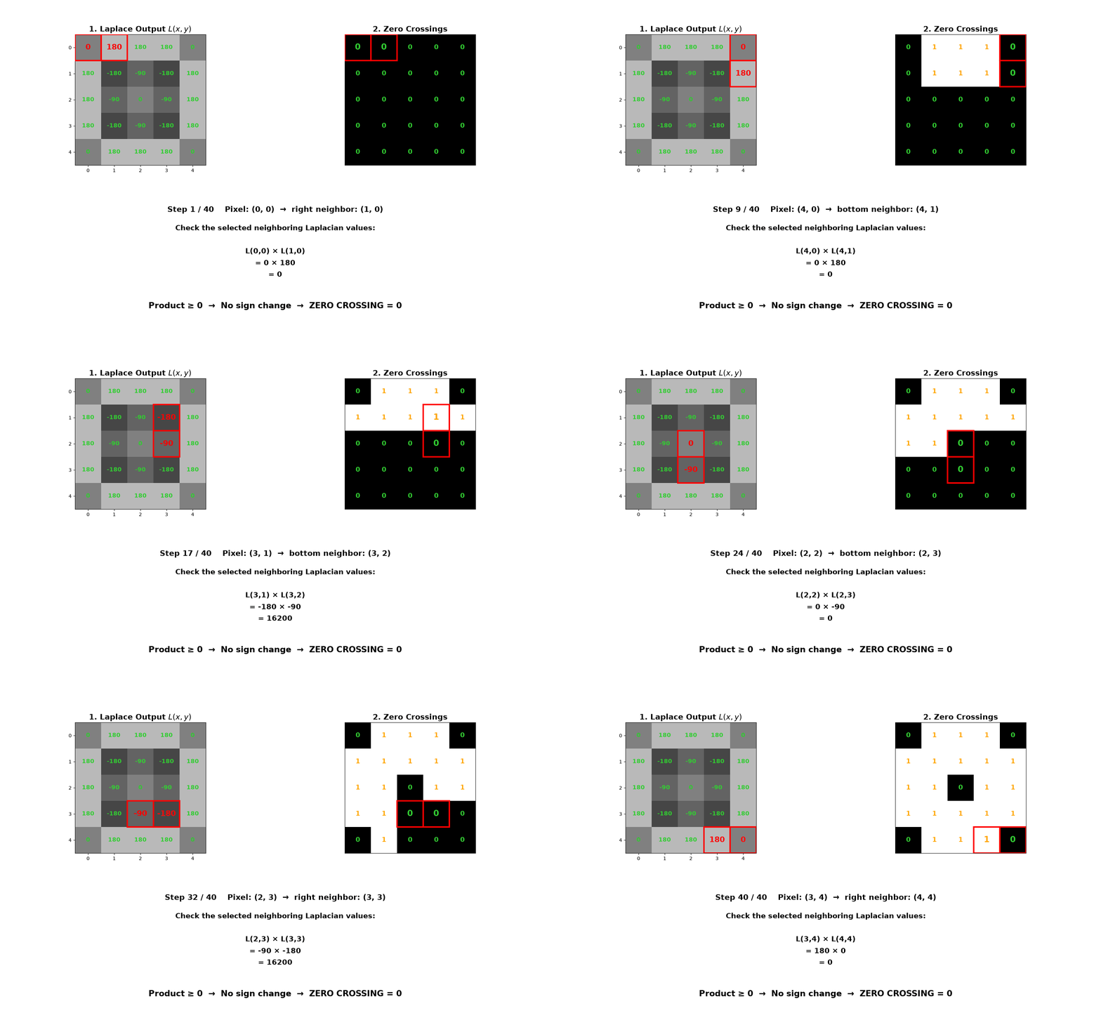
However, not every zero crossing represents a meaningful edge. Noise or very small intensity variations can also produce zero crossings, even after Gaussian smoothing.
The example below shows the detected zero crossings, before any thresholding, represented as a binary image.
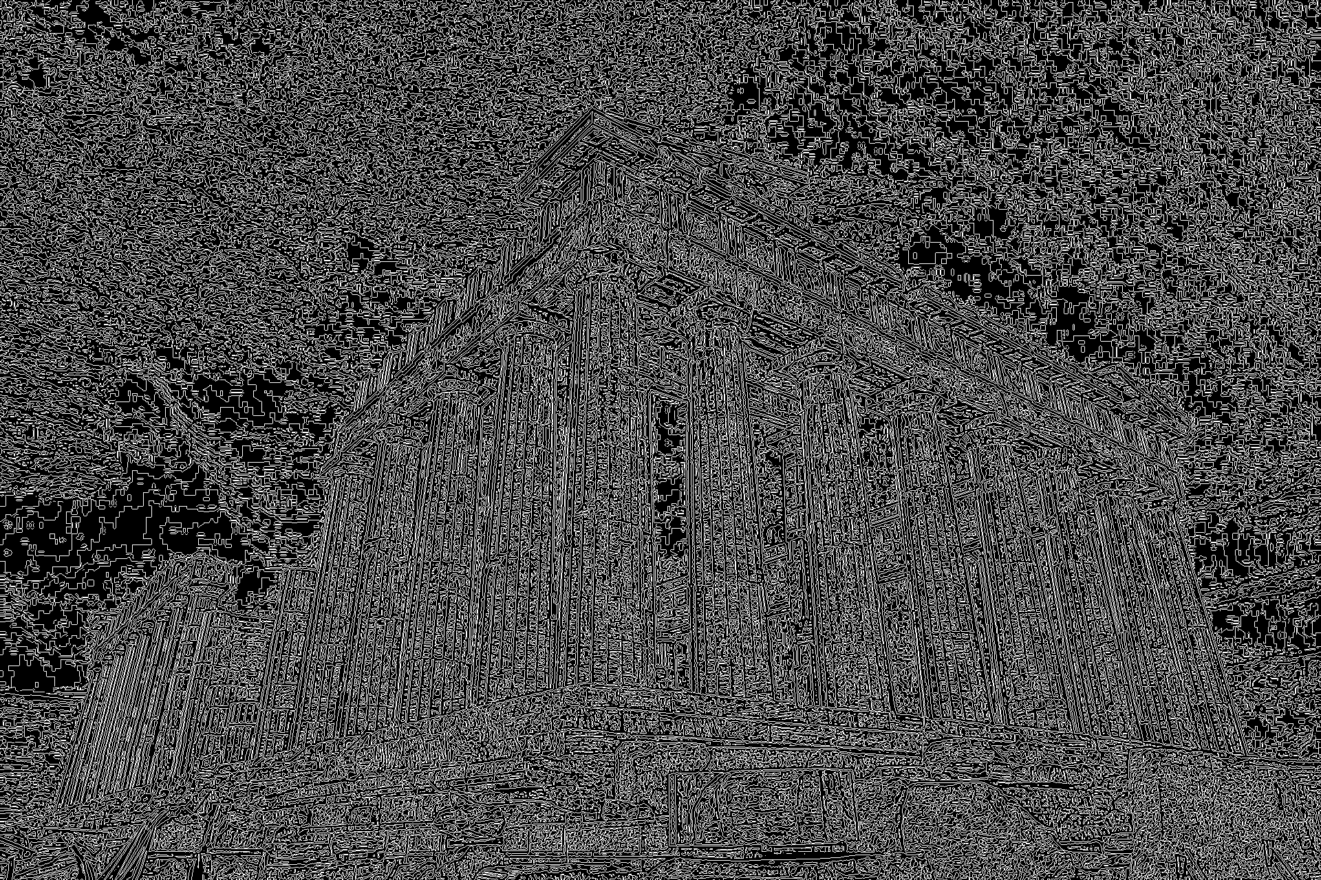
Step 5: Apply a Threshold
A threshold is applied to the detected zero crossings to remove weak responses caused by noise or insignificant intensity variations.
For each detected zero crossing, the Laplacian values of the two neighboring pixels that produced the sign change are compared. The absolute difference between these two values represents the strength of the zero crossing. Zero crossings with a strength below the selected threshold are discarded, while stronger zero crossings are retained.
Pixels that were not identified as part of a zero crossing are ignored during this step. The remaining zero crossings form the final binary edge image, where pixels corresponding to detected edges are typically represented as white and non-edge pixels as black.
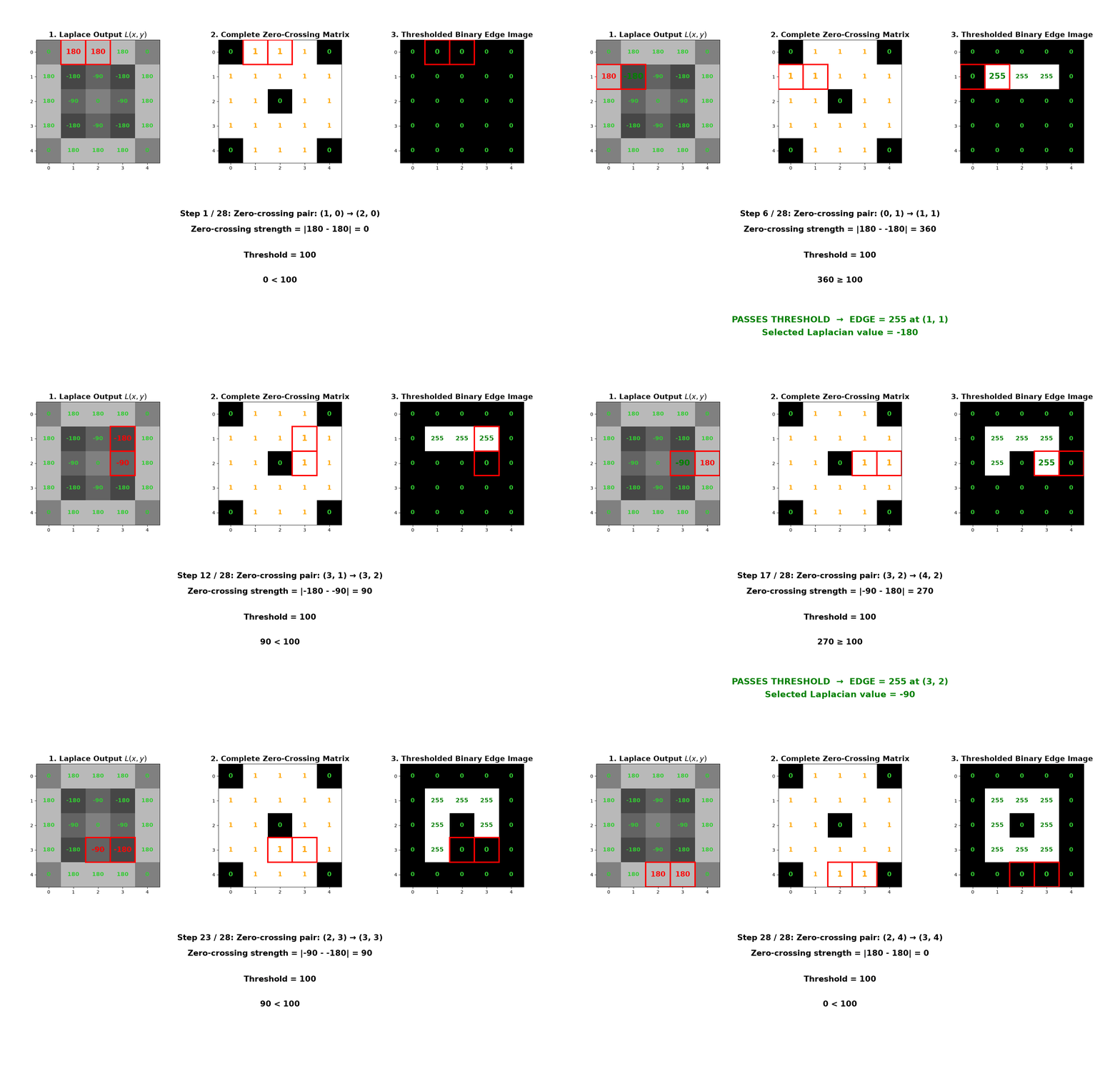
Depending on the implementation, once a zero crossing is determined to be strong enough to pass the threshold, the edge can be represented by one or both of the pixels involved in the zero crossing. An implementation may also estimate the edge location between the two pixels. In the example above, the pixel with the smaller Laplacian value is selected to represent the edge. Another implementation could instead select the pixel with the larger Laplacian value or use interpolation to estimate the edge location between them.
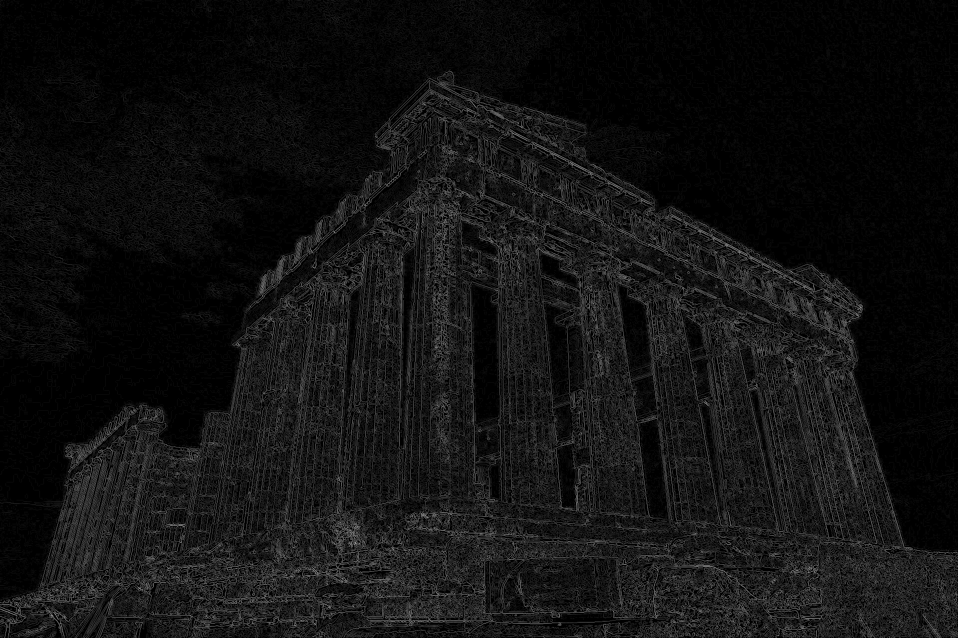
The example below shows the strength of each zero crossing, represented as a grayscale image.
The example below shows the resulting binary edge map after applying a threshold to the zero crossing strengths.
Sobel vs. Canny vs Laplacian Edge Detection
| Sobel | Canny | Laplacian | |
|---|---|---|---|
| Core Idea | Measures how fast intensity changes using first-order derivatives | Uses Sobel gradients in a multi-stage pipeline to produce clean, thin, connected edges | Detects where the second derivative of intensity changes sign |
| Main Steps | Grayscale → Sobel kernels → Gradient magnitude → Thresholding | Grayscale → Gaussian blur → Sobel gradients → Non-maximum suppression → Double threshold → Hysteresis | Grayscale → Gaussian blur → Laplacian kernel → Zero-crossing detection → Thresholding |
| Edge Detection | Detects edges from gradient magnitude calculated using horizontal and vertical gradients | Detects edges from Sobel gradient magnitude, then refines and connects them | Detects edges where the Laplacian changes sign between neighboring pixels |
| Direction Info | Yes: provides gradient magnitude and angle | Uses gradient direction internally for non-maximum suppression | No: the response is direction-independent |
| Edge Quality | Produces thicker and less precise edges | Produces thinner and more continuous edges | Can produce thin edges, but may detect unwanted zero crossings from small intensity variations |
| Thresholding | Threshold can be applied to the gradient magnitude when binary edge map required | Uses low and high thresholds with hysteresis | Applies a threshold to the strength of detected zero crossings to remove noise |
| Noise Sensitivity | Moderate: the Sobel kernel smooths neighboring pixels slightly, reducing some noise | Low: Gaussian blur reduces noise, while hysteresis removes weak and isolated edge responses | Highest: the second derivative is highly sensitive to noise, so Gaussian blur is essential to reduce noise before applying the Laplacian |
| Cost / Complexity | Lowest / simple | Highest / complex | Low-moderate / moderate |
| Output | Gradient-based edge map or thresholded binary edge image | Refined binary edge image | Thresholded binary edge image based on detected zero crossings |
| Best for | Quick gradient maps or applications where edge orientation matters | Clean, accurate edge maps | Precise edge localization when direction does not matter |
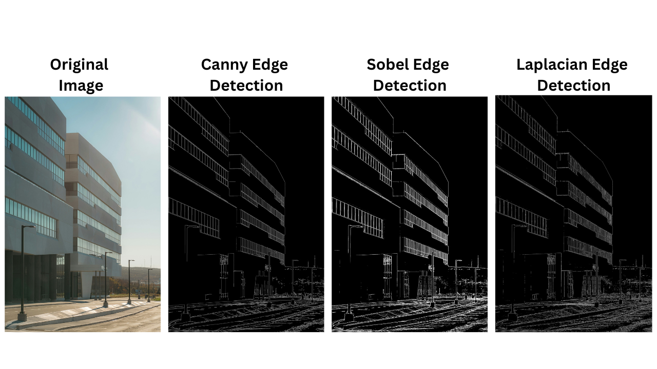
In the comparison below, Sobel produces thicker edges and captures more noise, especially around edge boundaries, while Canny produces thinner, more well-defined edges with significantly less noise, while Laplacian edge detection produces thin, sharp edges like Canny but is the very sensitive to noise.
Integrate Laplacian Edge Detection into Your Computer Vision Pipeline with Roboflow Workflows
You can integrate Laplacian Edge Detection into your computer vision pipeline using Roboflow Workflows. Workflows provides a range of pre-built blocks, including detection and segmentation models, image preprocessing, and visualization blocks. These blocks make it easy to build computer vision pipelines without having to implement every component from scratch.
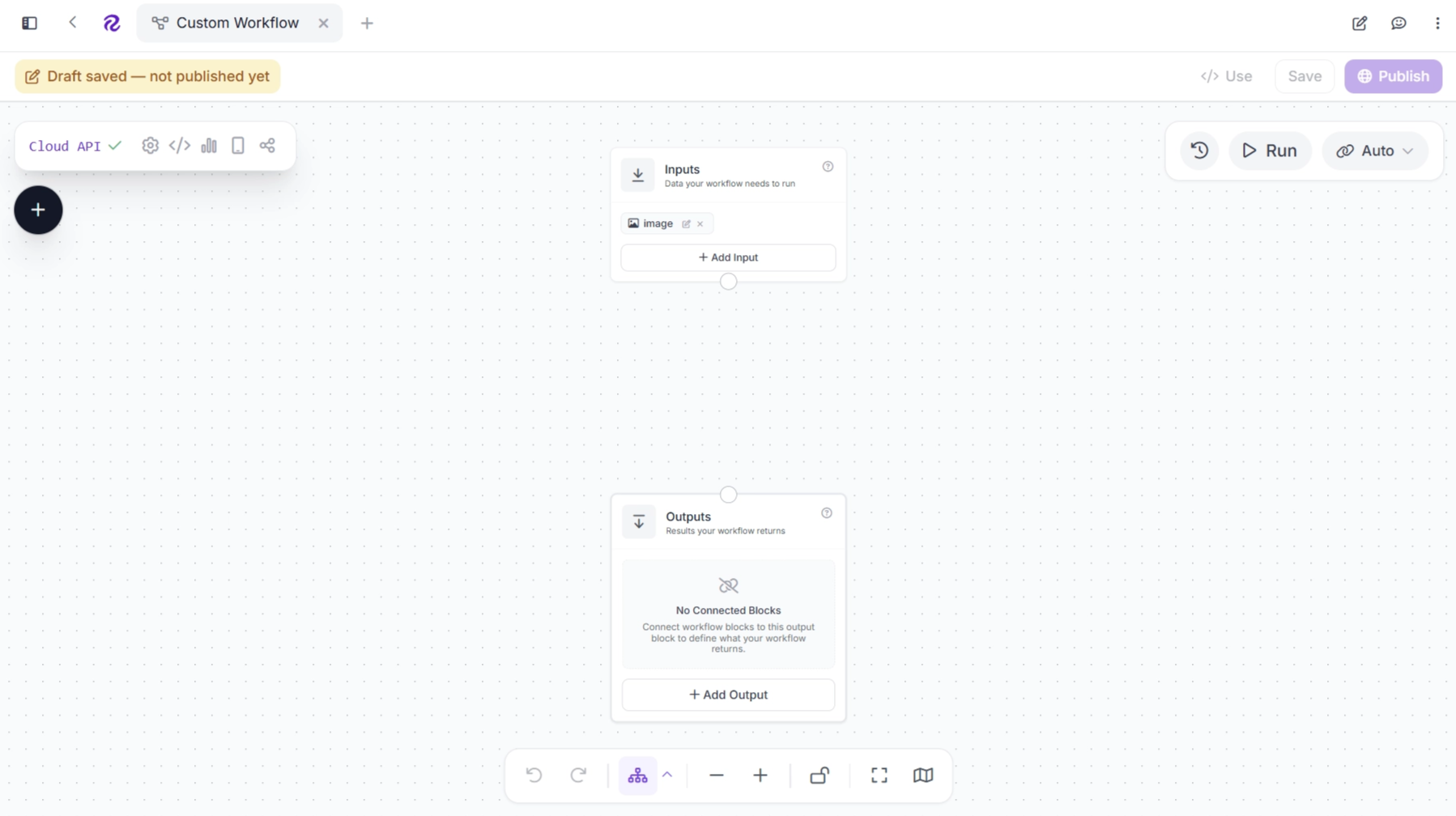
To build a Laplacian Edge Detection workflow, you can either create one manually in Roboflow or use Roboflow Agent. To create a workflow manually, log in to Roboflow, navigate to Workflows in the left sidebar, and select Create Workflow. This opens the Workflow Editor, where you can add and connect the blocks needed to build your pipeline.
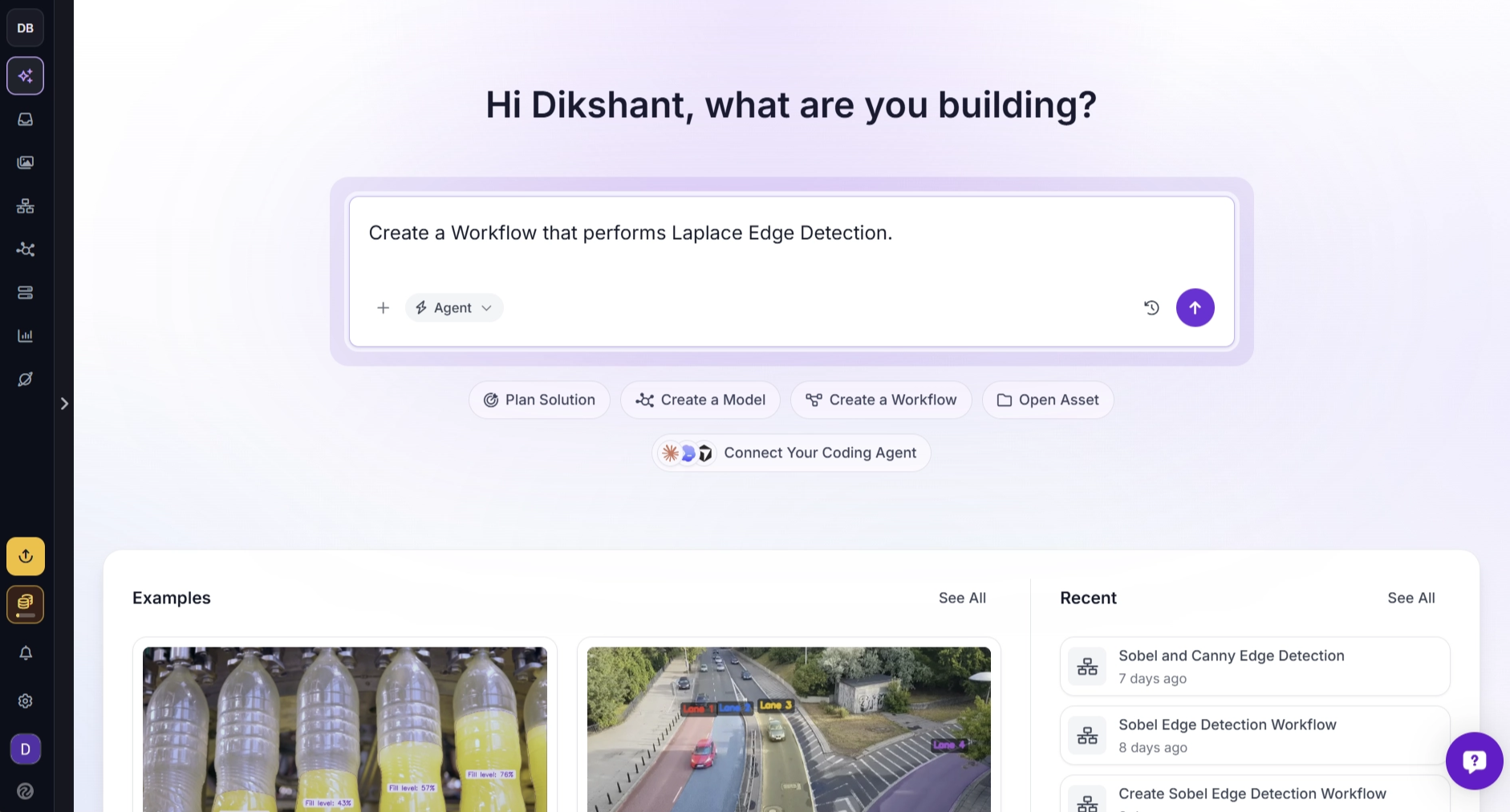
With Roboflow Agent (available after you log in), you can simply describe the workflow you want to create, and the Agent will build it for you. As shown below, I prompted the Agent to build a Laplacian Edge Detection workflow.
Roboflow Agent then generated a workflow that performed Laplacian Edge Detection on both images and video streams. It also provided an interface for testing the workflow by dragging and dropping images or videos into it.
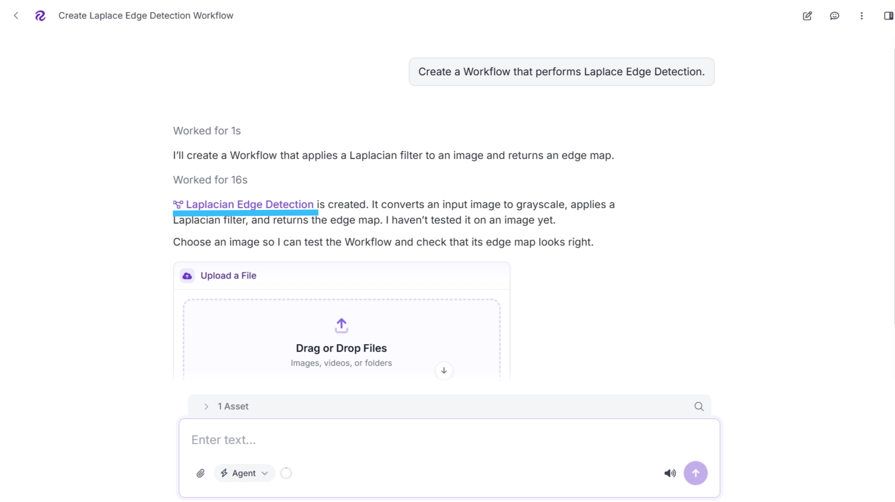
The interface shown below is accessible when you click the created workflow. You can also view the generated workflow from this interface.
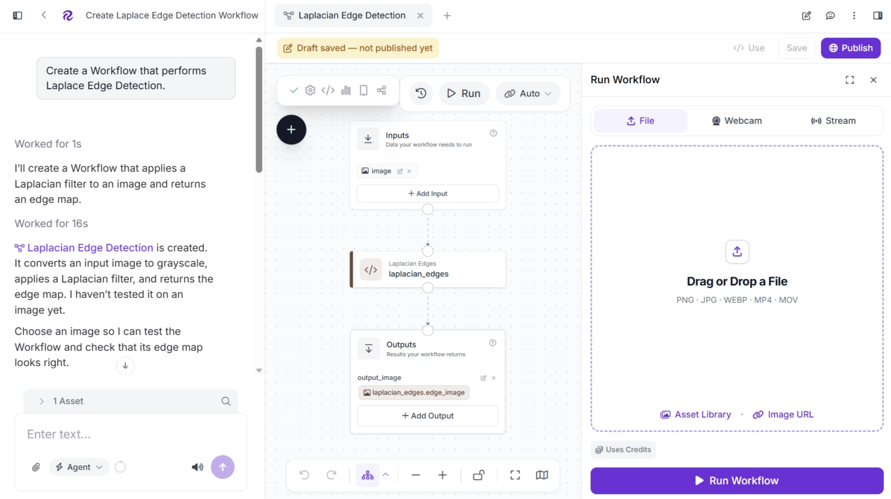
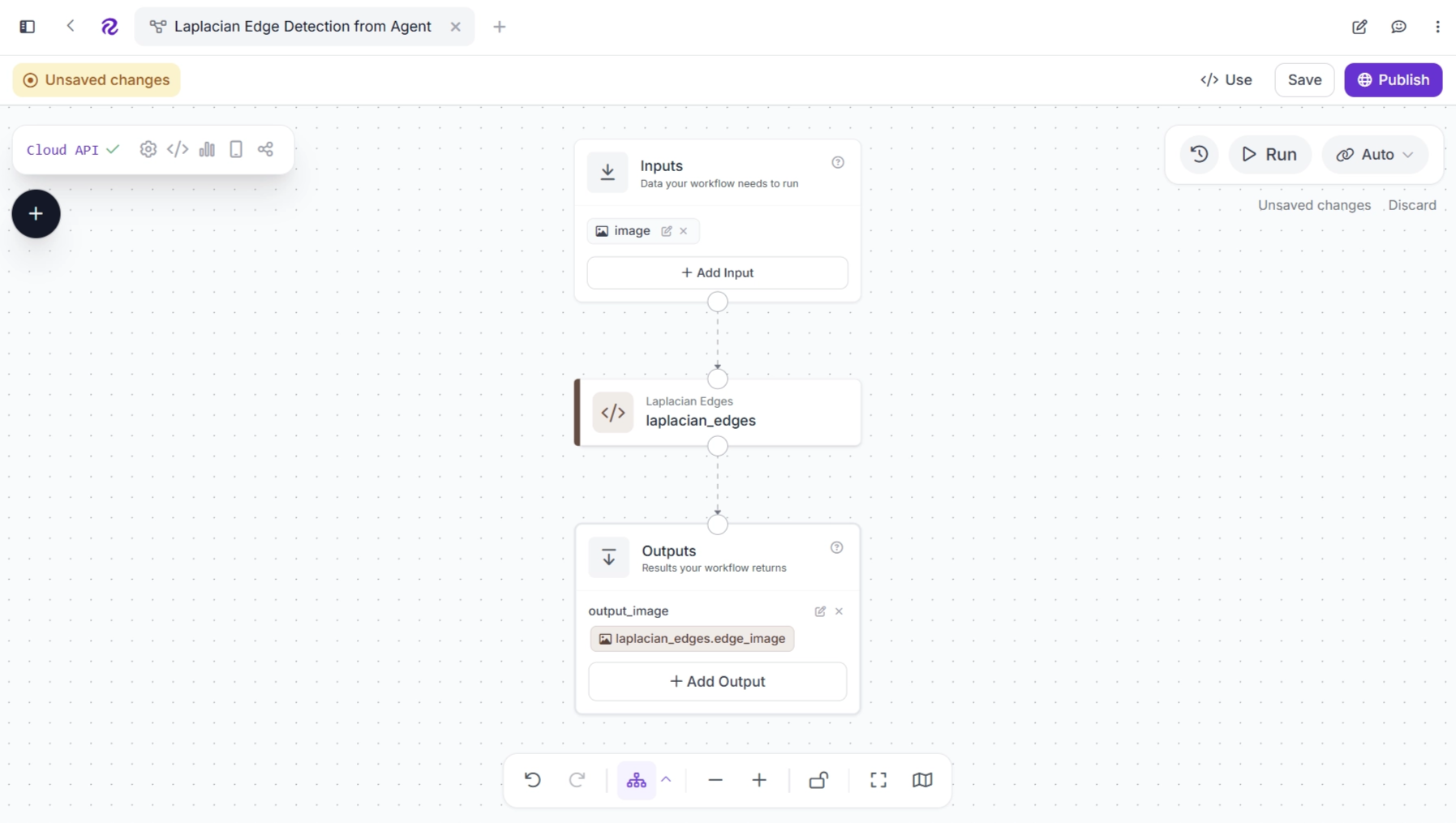
The generated workflow is shown below. It uses a Custom Python Block in Roboflow Workflows to implement Laplacian Edge Detection. Try the workflow.
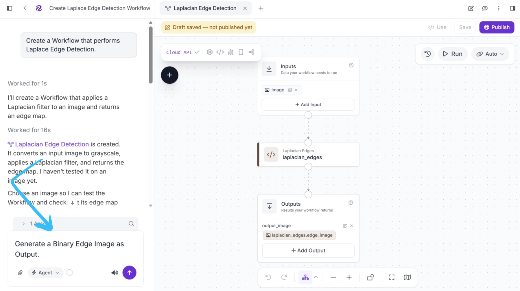
You can also use Roboflow Agent to add additional computer vision operations to the workflow. This allows you to build a complete computer vision workflow by describing the operations you want in a prompt.
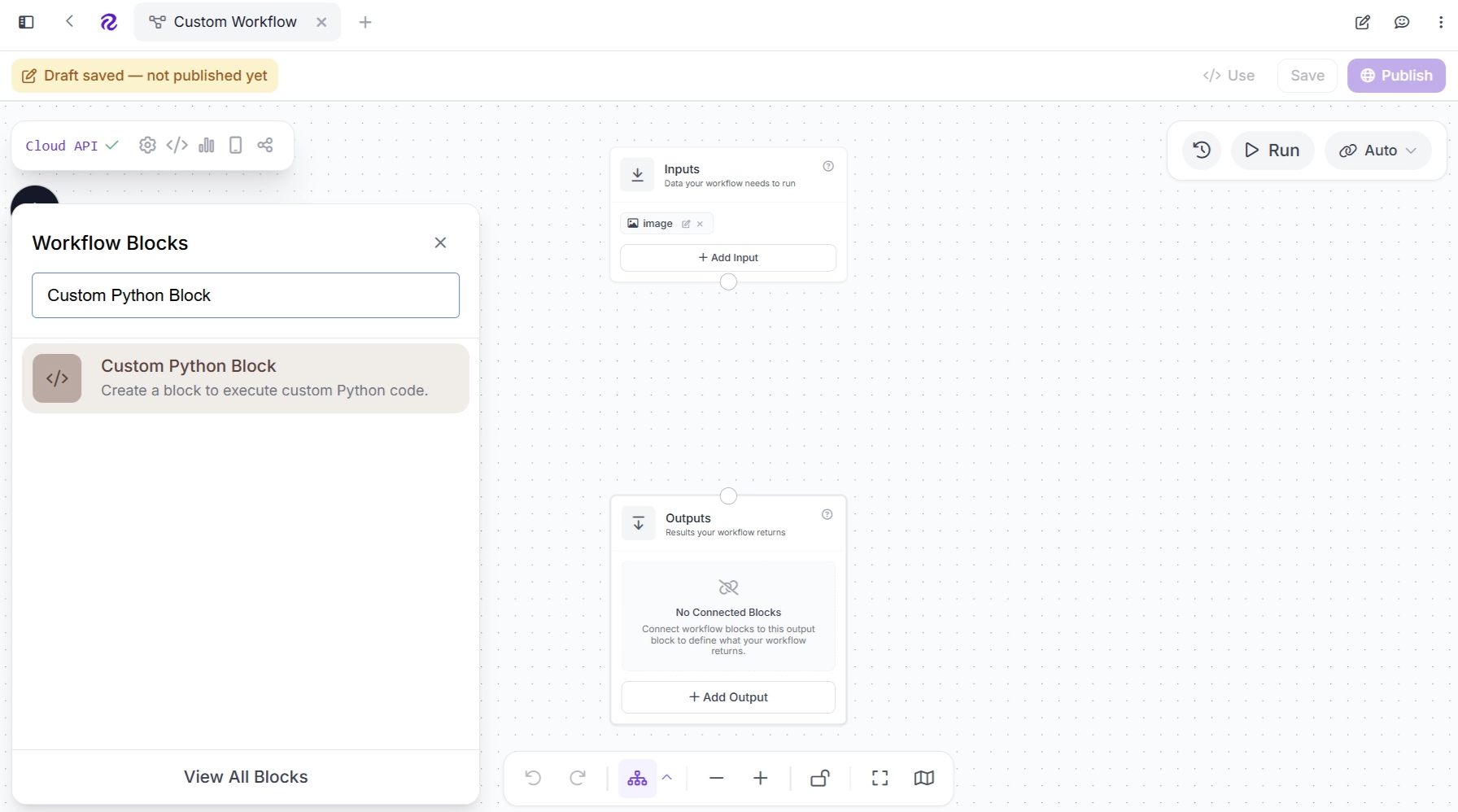
If you prefer to build the workflow manually, click the + button in the upper-left corner of the Workflow Editor, search for the Custom Python Block, and select it to add it to the workflow. Custom Python Blocks allow you to add your own Python code to a Workflow and use it alongside other workflow blocks.
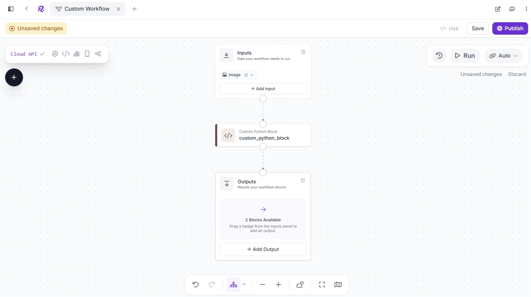
Once you add the block, connect it to the rest of the workflow as shown below.
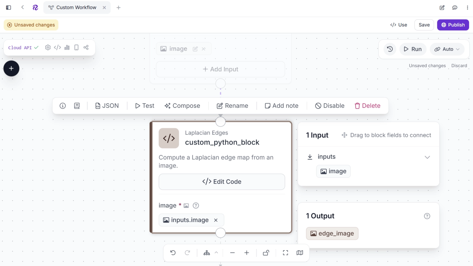
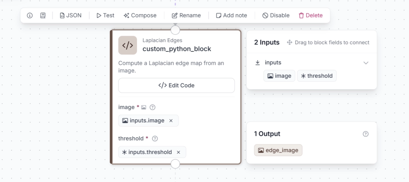
Next, select the Custom Python block and make sure its image parameter takes the image from the Inputs block. Then, click Edit Code to open the code editor, where you can configure the block and add your Python code.
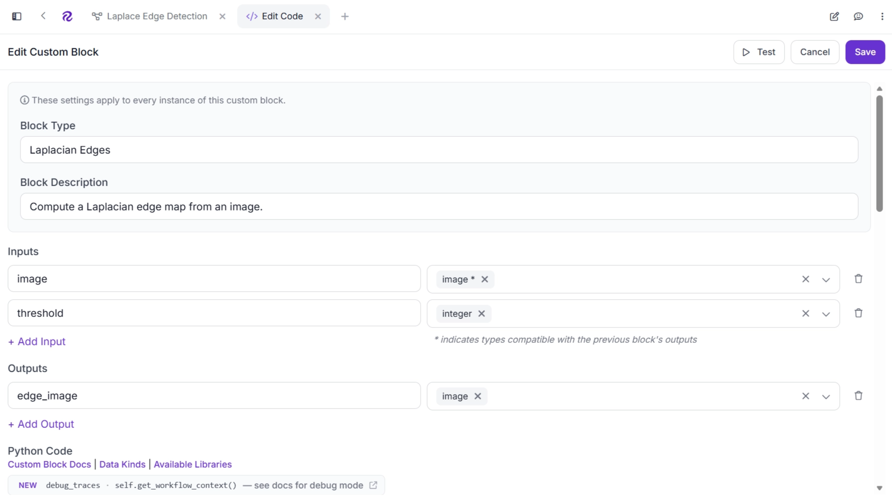
Then, Configure the Custom Python block as shown below:
In the Python Code section, add the following code. When you use Roboflow Agent, the code for this block is automatically generated.
import cv2
import numpy as np

def run(self, image, threshold):
    arr = image.numpy_image

    # Convert the image to grayscale
    if arr.ndim == 2:                 # already grayscale
        gray = arr
    elif arr.shape[2] == 4:           # color + alpha channel
        gray = cv2.cvtColor(arr, cv2.COLOR_BGRA2GRAY)
    elif arr.shape[2] == 3:           # normal color image
        gray = cv2.cvtColor(arr, cv2.COLOR_BGR2GRAY)
    else:
        gray = arr[:, :, 0]

    # Use decimal numbers so no precision is lost in the next steps
    gray = gray.astype(np.float32)

    # Apply Gaussian blur (reduces noise)
    blurred = cv2.GaussianBlur(gray, (5, 5), 0)

    # Apply the Laplacian kernel
    # Each pixel now holds a "second-order change" value (positive or negative)
    laplacian = cv2.Laplacian(blurred, cv2.CV_32F, ksize=3)

    # Detect zero crossings
    # Compare every pixel with its right neighbor and its bottom neighbor.
    # (Slicing lets us compare all pixels at once instead of using loops.)

    # Right-neighbor pairs: "current" is every pixel except the last column,
    # "right" is the same pixel shifted one column to the left.
    current_r = laplacian[:, :-1]
    right = laplacian[:, 1:]

    # Bottom-neighbor pairs: same idea, but moving down instead of right.
    current_b = laplacian[:-1, :]
    bottom = laplacian[1:, :]

    # A zero crossing = the two values have opposite signs,
    # so multiplying them gives a negative number.
    crossing_right = (current_r * right) < 0
    crossing_bottom = (current_b * bottom) < 0

    # Apply a threshold
    # Strength = how big the jump is between the two neighbors.
    strength_right = np.abs(current_r - right)
    strength_bottom = np.abs(current_b - bottom)

    # Keep only crossings that are strong enough
    # Zero crossings weaker than threshold are treated as noise
    strong_right = crossing_right & (strength_right >= threshold)
    strong_bottom = crossing_bottom & (strength_bottom >= threshold)

    # Build the final edge image
    # Start with an all-black image (0 = no edge)
    edges = np.zeros(laplacian.shape, dtype=np.uint8)

    # For each strong crossing, mark ONE of the two pixels as an edge:
    # the one with the smaller (more negative) Laplacian value.
    edges[:, :-1][strong_right & (current_r < right)] = 255   # left pixel
    edges[:, 1:][strong_right & (current_r >= right)] = 255   # right pixel

    edges[:-1, :][strong_bottom & (current_b < bottom)] = 255  # top pixel
    edges[1:, :][strong_bottom & (current_b >= bottom)] = 255  # bottom pixel

    # White pixels (255) are edges, black pixels (0) are not
    output = WorkflowImageData.copy_and_replace(
        origin_image_data=image,
        numpy_image=edges
    )

    return {
        'edge_image': output
    }
This code converts the input image to grayscale, applies Gaussian blur to reduce noise, and uses the Laplacian operator to calculate second-order intensity changes. It then detects zero crossings between neighboring pixels, filters them using a threshold to remove weak crossings, and marks the stronger crossings as edges to return a binary edge image.
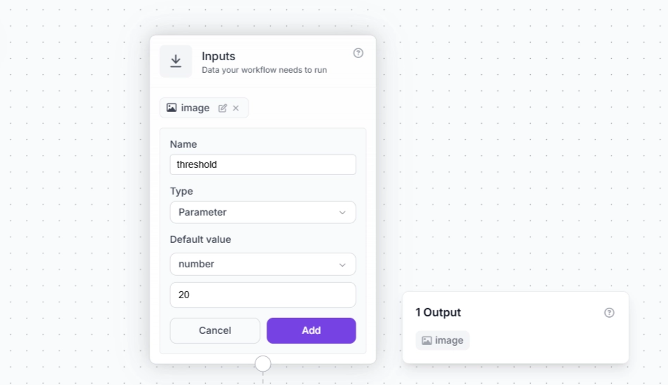
Since the code uses a threshold to determine which zero crossings are strong enough to be retained, add a threshold input parameter to the Inputs block. This allows the threshold to be provided as a workflow input. To do this, select the Inputs block and click + Add Input, as shown below.
Next, assign the threshold parameter from the Inputs block to the threshold parameter of the Custom Python block, as shown below.
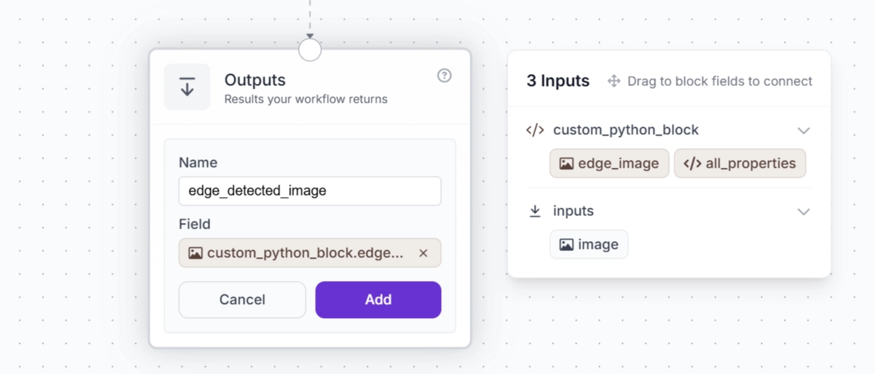
Finally, add an output parameter to the Outputs block. This output will represent the edge map generated by the Custom Python block and serve as the edge-detected image produced by the workflow. Select the Outputs block and click + Add Output, as shown below.
Your workflow should now look like the one shown below. You can then run the workflow directly from the Workflow Editor. Try the workflow.
Deploy Laplacian Edge Detection Workflows with Roboflow Deploy
Firstly, rename the workflow and make sure it is published. Giving the workflow an appropriate name makes it easier to identify and deploy, while publishing makes the workflow live and available through the API.
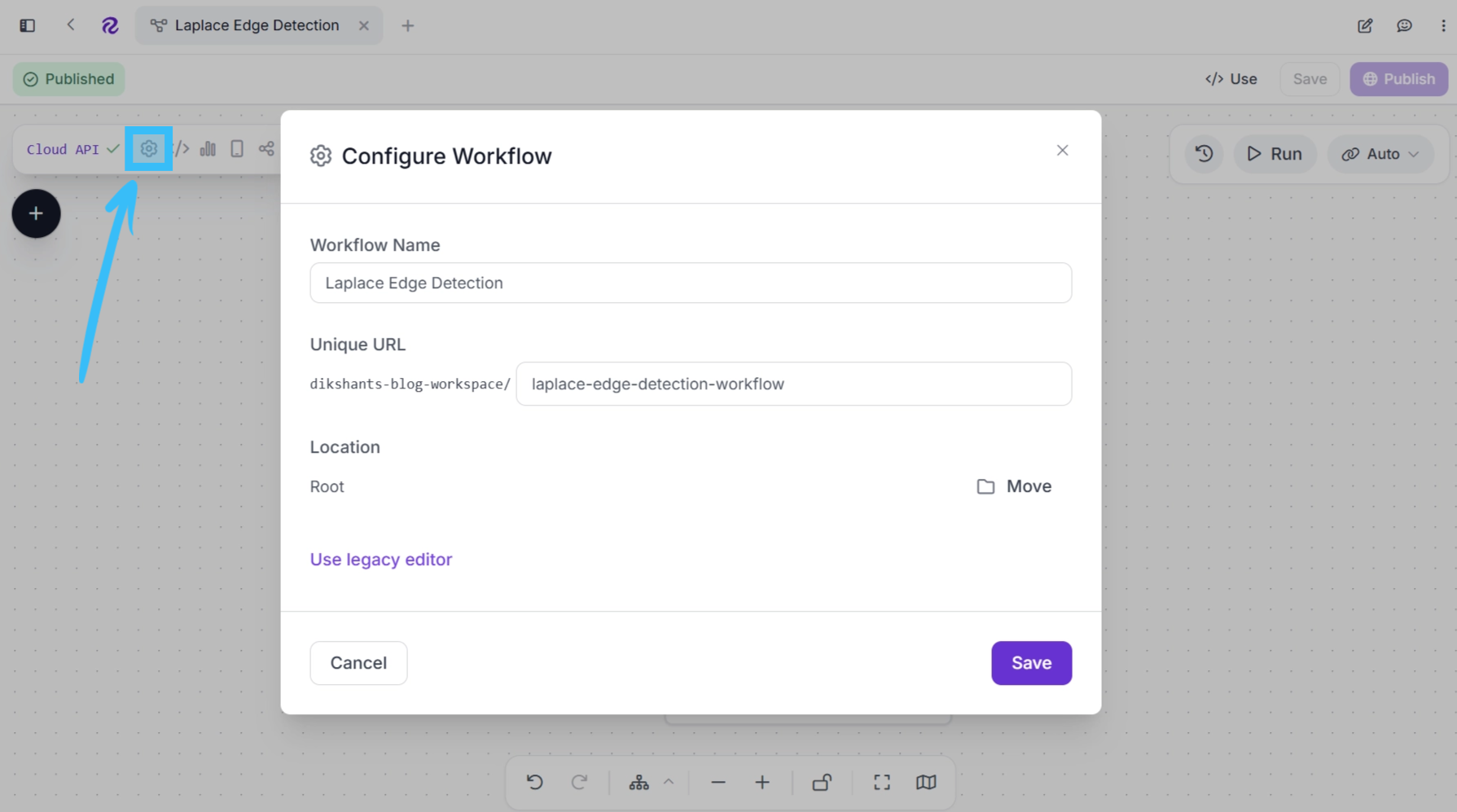
Once your edge detection workflow is published, click </> Use in the Workflows editor to open the deployment panel. From here, you can choose a deployment option and access everything you need to run your workflow in production.
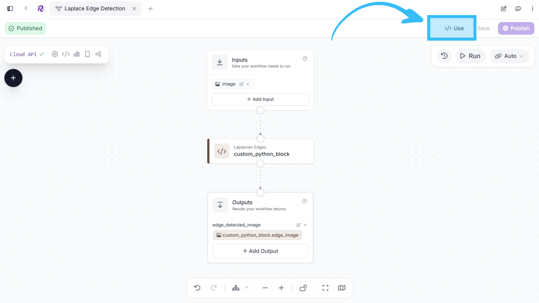
Roboflow Deploy automatically generates production-ready code snippets that you can copy directly into your application. These snippets can also be used with AI coding assistants such as Codex, Claude, Cursor, and ChatGPT to accelerate workflow integration and application development.

Roboflow Deploy also supports cloud-based deployment through the Serverless Cloud API, where your workflow runs in the cloud and you are charged credits for each inference.

You can also deploy your workflow locally and run it on your own hardware, including devices such as NVIDIA Jetson and Raspberry Pi.
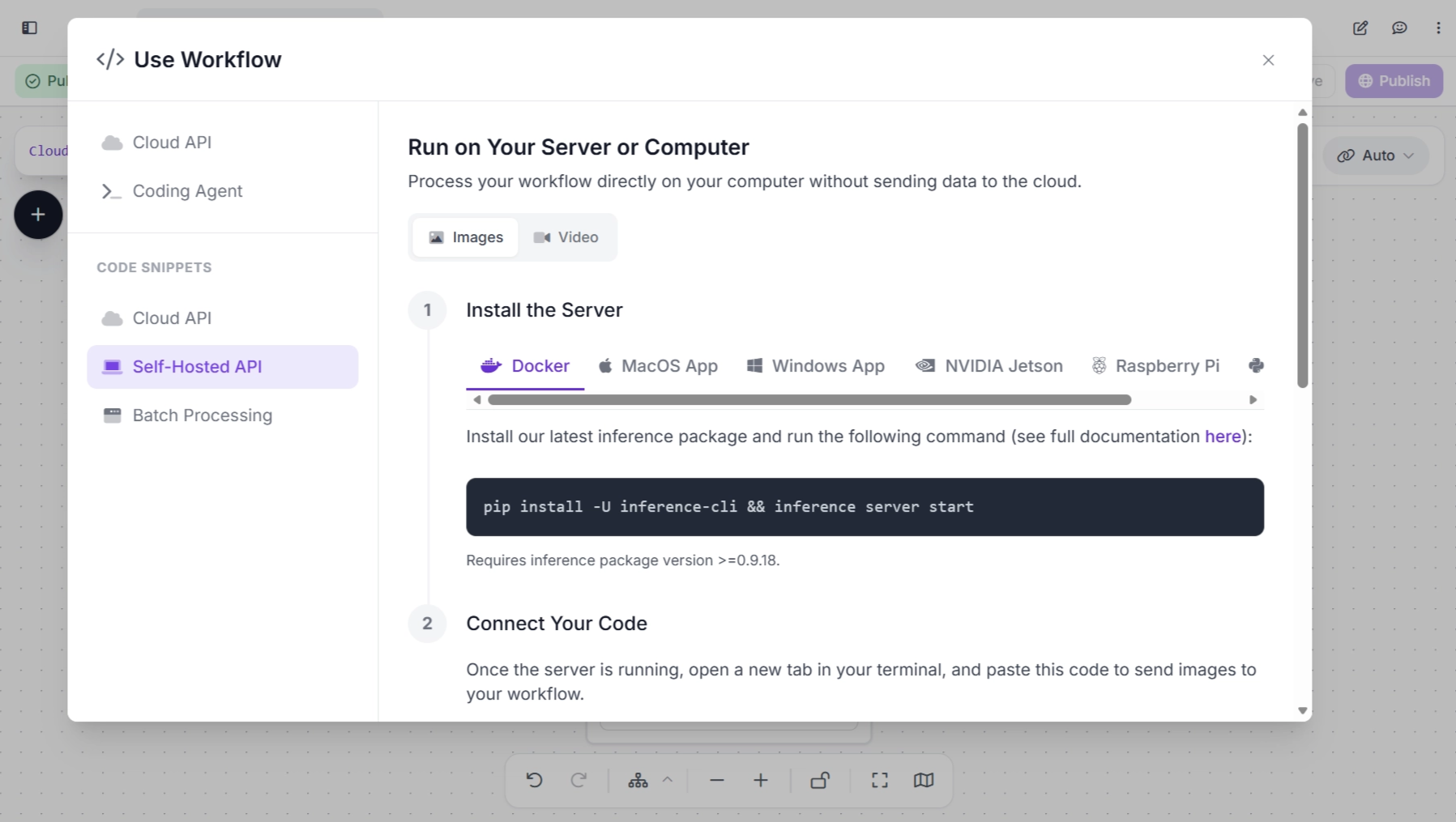
The Deployment panel provides ready-to-use code for running your workflow with different input sources, including images, video files, live webcam streams, and RTSP camera streams.
For example, the script below, provided by Roboflow Deploy, calls the Laplacian edge detection workflow with an input image and threshold parameter, then saves the output image locally:
import base64
from io import BytesIO
from PIL import Image
from inference_sdk import InferenceHTTPClient, InferenceConfiguration

# 2. Connect to your workflow
client = InferenceHTTPClient(
    api_url="https://serverless.roboflow.com",
    api_key="YOUR_ROBOFLOW_API_KEY"  # Replace with your actual API key
).configure(InferenceConfiguration(
    api_key_transport="header"  # header-based auth
))

# 2. Run your workflow
result = client.run_workflow(
    workspace_name="your-workspace", # Replace with your actual workspace name
    workflow_id="laplace-edge-detection-workflow",  # Replace with your actual workflow ID
    images={
        "image": "input.jpg" # Path to your image file
    },
    parameters={
        "threshold": 20
    },
    use_cache=True # Speeds up repeated requests
)

# 3. Get the Base64 image from the first result
output_image = result[0]["edge_detected_image"]

# 4. Decode the Base64 string
image_bytes = base64.b64decode(output_image)

# 5. Open the decoded image
image = Image.open(BytesIO(image_bytes))

# 6. Convert to RGB and save as JPEG
image.convert("RGB").save("laplace_output.jpg", "JPEG")

print("Saved output image as laplace_output.jpg")
Make sure you have installed the inference-sdk package before running the script above.
pip install -U inference-sdk
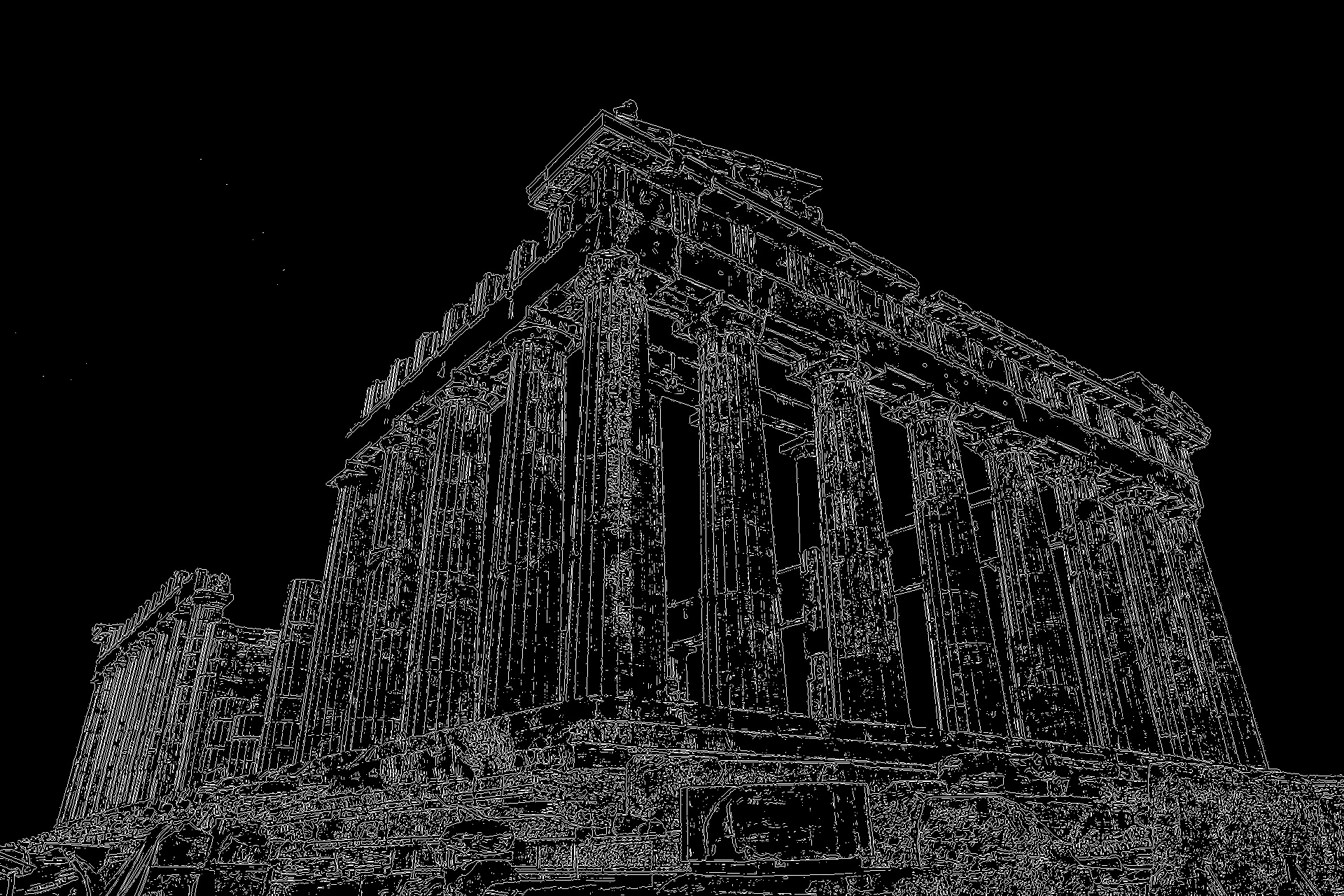
The image below shows the output image saved when you run the script:
Conclusion
Laplacian Edge Detection provides a easy way to identify edges by analyzing second-order changes in pixel intensity. Unlike Sobel Edge Detection, which calculates intensity changes separately in the horizontal and vertical directions before combining them, the Laplacian combines the second-order changes from both directions into a single response.
With the Roboflow Platform, Laplacian Edge Detection can become part of a larger computer vision pipeline without requiring you to build the surrounding infrastructure from scratch. Start building your own computer vision pipeline with Roboflow today.


Cite this Post
Use the following entry to cite this post in your research:
Dikshant Shah. (Sep 17, 2026). Laplacian Edge Detection in Computer Vision. Roboflow Blog: https://blog.roboflow.com/laplacian-edge-detection/