
This tutorial builds a computer vision application that reads a physical Connect 4 board and recommends the optimal next move using the minimax algorithm. An object detection model is trained on an annotated Connect 4 dataset from Roboflow Universe, deployed via Roboflow, and used to parse the board state from a camera frame. The detected piece positions are fed into minimax to evaluate future game states, and the recommended column is overlaid on the image with an arrow, demonstrating how computer vision and game-tree search can combine to drive real-time strategic decisions.
In this blog post, our goal is to explore the intersection of computer vision and game theory through the lens of a familiar classic: Connect 4.
We'll be crafting an application that uses computer vision to recognize Connect 4 pieces on the board and employs the minimax algorithm to predict the next best move. Below is an example of our algorithm in action, indicating where we (the yellow player) should drop our next token to maximize our chances of winning.
Beyond the realm of gaming, this blog offers a glimpse into the ever-expanding possibilities of computer vision and its potential to reshape data collection and decision making.
Without further ado, let’s walk through how this project works!
Step #1: Collect Data
If you already have data, skip to the next step!
First, we need to collect data relevant to our use case. Gathering data representative of your use case – and the environment in which your model will be deployed – is key to achieving high model performance.
You can search for data from Roboflow Universe, a community with over 200,000 computer vision datasets across different use cases.
Both of the above methods allow you to quickly gather data relevant to your use case that you can use for training the first version of your model.
For this guide, we are going to use a Connect 4 dataset from Roboflow Universe. This dataset contains annotated images of connect 4 boards and pieces, such as this one:
In the “Images” tab we can click “Select All” then “Clone 55 Select Images”. We will then choose the destination project below that we want to use for this project and “Import Images with Annotations”.
Step #2: Generate a Dataset Version
Once you have labeled all of your images, you can generate a dataset version. A dataset version is a frozen-in-time snapshot of your dataset.
You can apply preprocessing steps and augmentations to your dataset version. Preprocessing steps prepare your images for training. Augmentations let you generate new images using your dataset that may help improve model performance.
To generate a dataset version, click the “Generate” link in the left sidebar.
Click “Generate” at the bottom of the page to generate a dataset version. It will take a few moments for your dataset to be ready for use in training a model.
Step #3: Train an Object Detection model
With your dataset labeled and a dataset generated, you are ready to train your model. To do so, click the “Train with Roboflow” button on your dataset page.
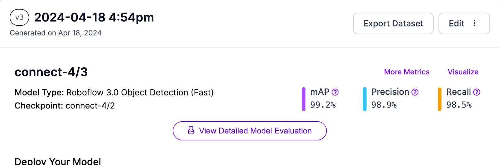
You can view the live performance of your training job from your dataset page and you will receive an email when the model is finished training.
Our model achieved training accuracy is 99.2%.
Step #4: Deploy your Connect 4 Model
You can deploy your Connect 4 model on your own hardware with Roboflow Inference. Inference is an open-source platform designed to simplify the deployment of computer vision models. It enables developers to perform object detection, classification, and instance segmentation and utilize foundation models like CLIP, Segment Anything, and YOLO-World through a Python-native package, a self-hosted inference server, or a fully managed API.
To deploy your model, first install inference_sdk and other dependencies that we will use including supervision and opencv-python:
!pip install -q supervision inference_sdk opencv-pythonWe can then write a script to run inference. Create a new file and add the following code:
# import the inference-sdk
from inference_sdk import InferenceConfiguration, InferenceHTTPClient
import cv2

image = cv2.imread("image.png")

# Define your custom confidence threshold (0.2 = 20%)
config = InferenceConfiguration(confidence_threshold=0.2)
# initialize the client
CLIENT = InferenceHTTPClient(
    api_url="https://detect.roboflow.com",
    api_key="API_KEY"
)

# infer on a local image
CLIENT.configure(config)
result = CLIENT.infer(image, model_id="connect-4/3")
print(result)
The above code gives output in JSON format as follows. This prediction result is stored in the result variable:
{'time': 0.05133835200012982, 'image': {'width': 822, 'height': 668}, 'predictions': [{'x': 206.5, 'y': 404.0, 'width': 49.0, 'height': 46.0, 'confidence': 0.9870650768280029, 'class': 'empty', 'class_id': 1, 'detection_id': '55b103e2-b189-4567-aaff-6fe409e6e261'}, {'x': 205.0, 'y': 346.5, 'width': 48.0, 'height': 47.0, 'confidence': 0.9870433211326599, 'class': 'empty', 'class_id': 1, 'detection_id': 'e4d22d2d-a4d9-4ddd-9529-7367b9eebe86'}, {'x': 592.0, 'y': 406.5, 'width': 48.0, 'height': 47.0, 'confidence': 0.9860526323318481, 'class': 'empty', 'class_id': 1, 'detection_id': 'c5f291cd-59a0-4f06-b5e7-0ae7f20d5540'}
...
]}
Step #5: Display Annotations and Labels
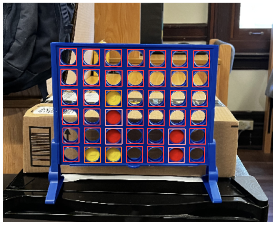
We’ll use the Supervision library to convert the results variable to draw bounding boxes and labels on our test image. Then we will use sv.plot_image to display our image.
import supervision as sv

detections = sv.Detections.from_inference(result)
# this model contains a "board" class (0), which we will want to exclude

detections = detections[detections.class_id != 0]
bounding_box_annotator = sv.BoundingBoxAnnotator()
annotated_frame = bounding_box_annotator.annotate(image, detections)

sv.plot_image(annotated_frame, (12, 12))
Here are the results of the bounding boxes from our model:
We can now use Supervision’s Label Annotator and the detections variable to create labels to display on the image that correspond to the classes identified by our model for each bounding box:
labels = [
    f"{class_name} {confidence:0.1f}"
    for class_name, confidence
    in zip(detections.data['class_name'], detections.confidence)
]

label_annotator = sv.LabelAnnotator(text_thickness=1, text_scale=.3)
annotated_frame = label_annotator.annotate(annotated_frame, detections, labels)

sv.plot_image(annotated_frame, (12, 12))
Here are the results plotted on an image:
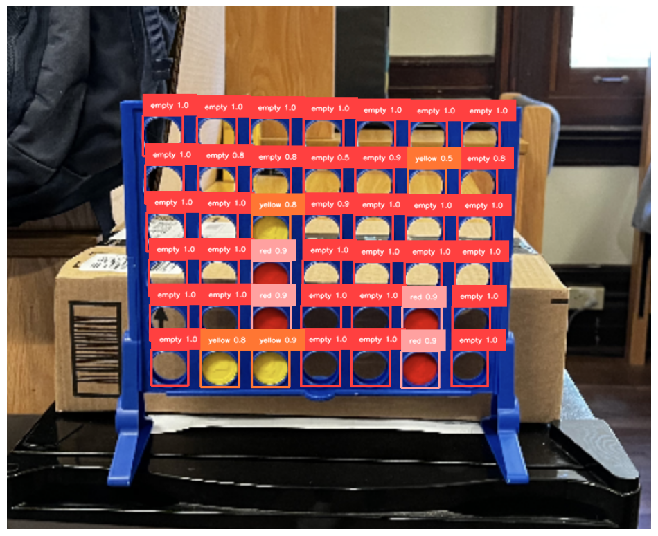
Let’s create a pieces variable that contains an array of all red, yellow, and empty slots. We will also check to make sure there are only 42 detections in this variable (6x7 board).
pieces = [p for p in result['predictions'] if p['class'] in ['red', 'yellow', 'empty']]
print(len(pieces))
if len(pieces) != 42:
    print("Incorrect amount of pieces detected!")
To create a digital representation of the board, let’s first sort pieces by the value of the 'y' key in ascending order to create a new list sorted_pieces. Next we will group this sorted list into smaller sublists of seven elements each. Lastly, for each of these subgroups, let’s perform another sort, this time by the 'x' key in ascending order, and collect these fully sorted subgroups into a new list fully_sorted.
# Sort the list of dictionaries by the 'y' value
sorted_pieces = sorted(pieces, key=lambda d: d['y'], reverse=False)
grouped_data = [sorted_pieces[i:i + 7] for i in range(0, len(sorted_pieces), 7)]

fully_sorted = []
for group in grouped_data:
    sorted_group = sorted(group, key=lambda d: d['x'], reverse=False)
    fully_sorted.append(sorted_group)
Step #6: Implementing the Minimax Algorithm
For the solving piece of this blog, we will be mimicking this website post on utilizing the minimax algorithm on this website. The minimax algorithm is a decision-making tool used in artificial intelligence (AI) for minimizing the possible loss for a worst case (maximum loss) scenario. When applied to games like Connect 4, the algorithm plays out all possible moves on the board, forecasts the outcomes, and chooses the move that maximizes the player's chances of winning while minimizing the opponent's best playing options.
This recursive algorithm evaluates the game state from the terminal nodes of a game tree, based on a scoring function. It alternates between minimizing and maximizing the scores, hence the name 'minimax', to decide the optimal move for the player. This strategy is particularly effective in Connect 4 because it can exhaustively explore all possible game states due to the game’s limited complexity and board size.
We first need to build a board variable that will act as a supported input variable for the algorithm:
def build_board(fully_sorted):
    board  = []
    for row in fully_sorted:
        each_row = []
        for col in row:
            each_row.append(col['class_id'])
        board.append(each_row)
    return board
board = (build_board(fully_sorted))
print(board)
The output is:
[[1, 1, 1, 1, 1, 1, 1], [1, 1, 1, 1, 1, 3, 1], [1, 1, 3, 1, 1, 1, 1], [1, 1, 2, 1, 1, 1, 1], [1, 1, 2, 1, 1, 2, 1], [1, 3, 3, 1, 1, 2, 1]]
The board variable represents a 6x7 grid for a Connect 4 game board, where each number corresponds to a cell status: '1' for empty, '2' for a red piece, and '3' for a yellow piece.
OPPONENT_PIECE = 3  # Assuming opponent is red
MY_PIECE = 2  # Assuming you are yellow
EMPTY = 1  # Empty cells
row_count = len(board)
column_count = len(board[0])


# To get all locations in the board that could contain a piece (i.e. have not yet been filled):
def get_valid_locations(board):
   return [col for col in range(column_count) if board[0][col] == EMPTY]


# To check if there is a valid location in the chosen column:
def is_valid_location(board, col):
    return board[ROW_COUNT - 1][col] == 0


#check if a winning move has been made
def is_winner(board, piece):
     # Horizontal check
    for c in range(column_count - 3):  # Subtract 3 to avoid out-of-bounds
        for r in range(row_count):
            if board[r][c] == piece and board[r][c + 1] == piece and board[r][c + 2] == piece and board[r][c + 3] == piece:
                return True

    # Vertical check
    for c in range(column_count):
        for r in range(row_count - 3):  # Subtract 3 to avoid out-of-bounds
            if board[r][c] == piece and board[r + 1][c] == piece and board[r + 2][c] == piece and board[r + 3][c] == piece:
                return True

    # Positive diagonal check
    for c in range(column_count - 3):
        for r in range(row_count - 3):
            if board[r][c] == piece and board[r + 1][c + 1] == piece and board[r + 2][c + 2] == piece and board[r + 3][c + 3] == piece:
                return True

    # Negative diagonal check
    for c in range(column_count - 3):
        for r in range(3, row_count):
            if board[r][c] == piece and board[r - 1][c + 1] == piece and board[r - 2][c + 2] == piece and board[r - 3][c + 3] == piece:
                return True

    return False

#To check which row the piece can be placed into (i.e. the next available open row):
def get_next_open_row(board, col):
   for r in range(row_count-1, -1, -1):
       if board[r][col] == EMPTY:
           return r
   return None


# to place a piece in the next available row, in the chosen column:
def drop_piece(board, row, col, piece):
   board[row][col] = piece


# evaluates a Connect 4 board by scanning and scoring all possible four-piece lineups in various directions to predict the next best move.
def score_position(board, piece):
   score = 0
   center_index = column_count // 2

   # Score center column (more opportunities if more pieces are in the center)
   center_array = [board[r][center_index] for r in range(row_count)]
   center_count = center_array.count(piece)
   score += center_count * 3

   # Score Horizontal
   for r in range(row_count):
       row_array = board[r]
       for c in range(column_count - 3):
           window = row_array[c:c+4]
           score += evaluate_window(window, piece)

   # Score Vertical
   for c in range(column_count):
       col_array = [board[r][c] for r in range(row_count)]
       for r in range(row_count - 3):
           window = col_array[r:r+4]
           score += evaluate_window(window, piece)

   # Score positive diagonal
   for r in range(row_count - 3):
       for c in range(column_count - 3):
           window = [board[r+i][c+i] for i in range(4)]
           score += evaluate_window(window, piece)

   # Score negative diagonal
   for r in range(3, row_count):
       for c in range(column_count - 3):
           window = [board[r-i][c+i] for i in range(4)]
           score += evaluate_window(window, piece)

   return score

# provides a score based on piece configuration, awarding higher points for sequences closer to a win, and adjusts scores to prioritize potentially winning or blocking moves in the Connect 4 game.
def evaluate_window(window, piece):
    score = 0
    opp_piece = OPPONENT_PIECE if piece == MY_PIECE else MY_PIECE

    if window.count(piece) == 4:
        score += 100
    elif window.count(piece) == 3 and window.count(EMPTY) == 1:
        score += 5
    elif window.count(piece) == 2 and window.count(EMPTY) == 2:
        score += 2

    if window.count(opp_piece) == 3 and window.count(EMPTY) == 1:
        score -= 4

    return score


#this function recursively calculates the optimal move in a game by exploring potential future states, considering maximizing or minimizing outcomes, and using alpha-beta pruning to enhance efficiency
import random
def minimax(board, depth, alpha, beta, maximizingPlayer):
   valid_locations = get_valid_locations(board)
   is_terminal = is_winner(board, MY_PIECE) or is_winner(board, OPPONENT_PIECE) or len(valid_locations) == 0
   if depth == 0 or is_terminal:
       if is_terminal:
           if is_winner(board, MY_PIECE):
               return (None, float('inf'))
           elif is_winner(board, OPPONENT_PIECE):
               return (None, float('-inf'))
           else:  # Game is over, no more valid moves
               return (None, 0)
       else:  # Depth is zero
           return (None, score_position(board, MY_PIECE if maximizingPlayer else OPPONENT_PIECE))

   if maximizingPlayer:
       value = float('-inf')
       column = random.choice(valid_locations)  # Default to a random choice
       for col in valid_locations:
           row = get_next_open_row(board, col)
           temp_board = [x[:] for x in board]
           drop_piece(temp_board, row, col, MY_PIECE)
           new_score = minimax(temp_board, depth-1, alpha, beta, False)[1]
           if new_score > value:
               value = new_score
               column = col
           alpha = max(alpha, value)
           if alpha >= beta:
               break
       return column, value
   else:
       value = float('inf')
       column = random.choice(valid_locations)
       for col in valid_locations:
           row = get_next_open_row(board, col)
           temp_board = [x[:] for x in board]
           drop_piece(temp_board, row, col, OPPONENT_PIECE)
           new_score = minimax(temp_board, depth-1, alpha, beta, True)[1]
           if new_score < value:
               value = new_score
               column = col
           beta = min(beta, value)
           if beta <= alpha:
               break
       return column, value


#call evaluates the board to determine the best column (best_col) to play and the associated value (best_val)
best_col, best_val = minimax(board, 8, float('-inf'), float('inf'), True)  # Assume it’s your turn
print(best_col, best_val)
In the code above:
- best_col: This is the column index (4th column) where the minimax algorithm determines you should place your next move for optimal strategy based on the current state of the board and looking eight moves ahead.
- best_val: indicates how favorable or unfavorable the board position is predicted to be after making the move in best_col, given all subsequent optimal plays up to eight moves deep.
For the image we showed earlier, our code returns:
3, 203 is the best column in which to play. We can plot it on our original image to make the results easier to interpret. We will do this in the next section.
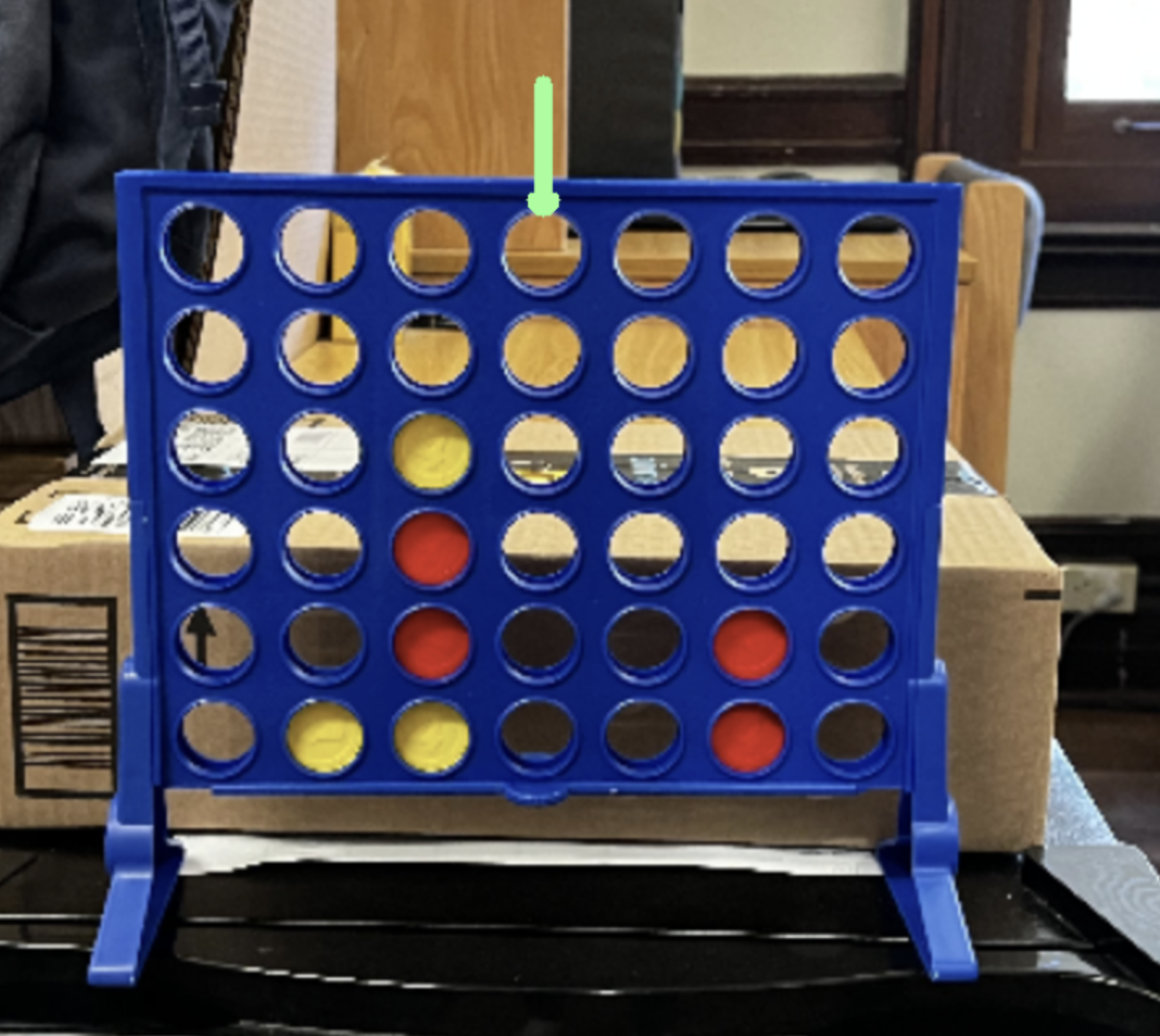
Step #7: Display your next best move
To finish plotting where the next best move will be for our turn, we’ll need to define a variable that contains the x, y, and height component for the top row of pieces identified in our image:
column_values = [(item['x'], item['y'], item['height']) for item in sorted_pieces[0:7]]
print(column_values)


[(198.5, 165.0, 52.0), (267.5, 166.5, 51.0), (335.5, 168.0, 52.0), (403.5, 169.0, 52.0), (470.0, 170.5, 51.0), (537.0, 171.0, 50.0), (604.0, 171.5, 51.0)]
With this information, we can utilize the OpenCV library to plot and arrow downwards of the slot we should place our piece:
image = cv2.imread("image2.png")
copy = image.copy()

end_point = (int(column_values[best_col][0]), int((column_values[best_col][1])-(column_values[best_col][2])/2))
start_point = (int(end_point[0]), int(end_point[1])-75)
color = (150,255,150)

thickness = 10
image = cv2.arrowedLine(image, start_point, end_point, color, thickness)
sv.plot_image(image,(12,12))
Our code returns:
The next best move for us will be the 4th column from the left. Therefore, no matter where the opponent (red) moves on their next turn, we can win the game.
Conclusion
The integration of computer vision into Connect 4 is not just about stepping up the competition; it's about reshaping our entire approach to the game. By allowing machines to see and analyze the board just like a human player, it revolutionizes how we interact with and strategize in the game.
This technology brings us smarter gameplay, deeper insights, and a fresher way to enjoy an old favorite. As computer vision technology keeps advancing, it's set to transform our Connect 4 experiences into something more interactive and insightful, blending the charm of classic gameplay with the excitement of modern tech.
Cite this Post
Use the following entry to cite this post in your research:
Nathan Marraccini. (May 8, 2024). Predicting the Optimal Connect 4 Move with Computer Vision. Roboflow Blog: https://blog.roboflow.com/connect-4-computer-vision/