How to Evaluate Computer Vision Models with CVevals

Metrics surrounding the performance of your computer vision model – from precision to recall to mAP – form the basis of many important decisions one has to make during the process of building a model. Using model metrics, you can answer questions like:

• Is my model ready for production?
• Is the false positive rate too high?
• How does the newest iteration of my model compare to previous ones?

Using Roboflow’s open-source CVevals package, you can evaluate object detection and classification models hosted on Roboflow.

CVevals compares the ground truth in your dataset – the annotations you have added to images – with predictions your model yields on images in your validation dataset and uses that information to calculate evaluation metrics on your dataset.

In this guide, we’re going to show how to use CVevals to evaluate a retail shelf object detection dataset. By the end of this tutorial, we will have metrics on precision, recall, F1, and a confusion matrix showing how our model performs on our validation dataset. We'll also review, briefly, how to run an evaluation on a classification dataset.

We can use these metrics to make a decision on whether a model is ready for production and, if it is not, provide data on what we may need to do to improve our model to prepare it for production.

Without further ado, let’s get started!

Step 1: Install CVevals

The CVevals package is bundled in a Github repository. This repository contains many examples showing how to evaluate different types of models, from Roboflow models to state-of-the-art zero-shot models such as Grounding DINO and CLIP. For this guide, we’ll focus on the example for evaluating a Roboflow model.

To install CVevals, run the following lines of code:

git clone https://github.com/roboflow/evaluations.git
cd evaluations
pip install -r requirements.txt
pip install -e .

This code will download the package and install it on your local machine. Now we’re ready to start evaluating our model!

Step 2: Configure the Evaluation

Suppose we’re working with a retail shelfobject detection model that finds empty spaces on a shelf and spaces where a product is present. We want to know how many false positives the model returns on our validation dataset. We also want to be able to visualize the bounding boxes returned by our model. We can accomplish both of these tasks using CVevals.

CVevals works in three stages:

1. You specify a source from which to load your ground truth data;
2. You specify a source from which to load model predictions (in this example, we’ll use Roboflow);
3. The ground truth data is compared with predictions to calculate evaluation metrics.

In this example, we can use the examples/roboflow_example.py script. This script loads data from Roboflow and runs your model on your validation dataset.

To use the script, you will need your:

1. Roboflow API key
2. Workspace ID
3. Model ID
4. Model version number

You can learn how to retrieve these values in our documentation.

We also need to choose a location where we will store the data we’ll use in our evaluation. We recommend storing the data in a new folder. For this guide, we’ll store data on this path:

/Users/james/cvevals/retail-shelf-data/

If the folder doesn’t already exist, it will be created.

Now we’re ready to run our evaluation!

Step 3: Run the Evaluation

To run the evaluation, use the following command:

python3 examples/roboflow_example.py --eval_data_path=<path_to_eval_data> \
--roboflow_workspace_url=<workspace_url> \
--roboflow_project_url=<project_url> \
--roboflow_model_version=<model_version>
--model_type=object-detection

Substitute the values you noted in the last section in the angle brackets above. Then, run the command.

If you are working with a single-label classification dataset, set the --model_type= value to classification. If you are working with a multi-label classification dataset, use --model_type=multiclass.

This code will: (i) retrieve your ground truth data, in this case from Roboflow; (ii) run inference on each image in your validation set; (ii) return prediction results. As inference runs on each image, a message will be printed to the console like this:

evaluating image predictions against ground truth <image_name>

The amount of time the evaluation script takes will depend on how many validation images you have in your dataset.

After the evaluation is finished, you will see key metrics printed to the console, like this:

Precision: 0.7432950191570882
Recall: 0.8083333333333333
f1 Score: 0.7744510978043913

There will also be a new folder on your computer called `output` that contains two subfolders:

1. matrices: Confusion matrices for each image in your dataset.
2. images: Your images with ground truth and model predictions plotted onto the image.

There is a special matrix called aggregate.png which reflects the performance of your model across all images in your dataset. Here is what the confusion matrix looks like for our retail shelf example:

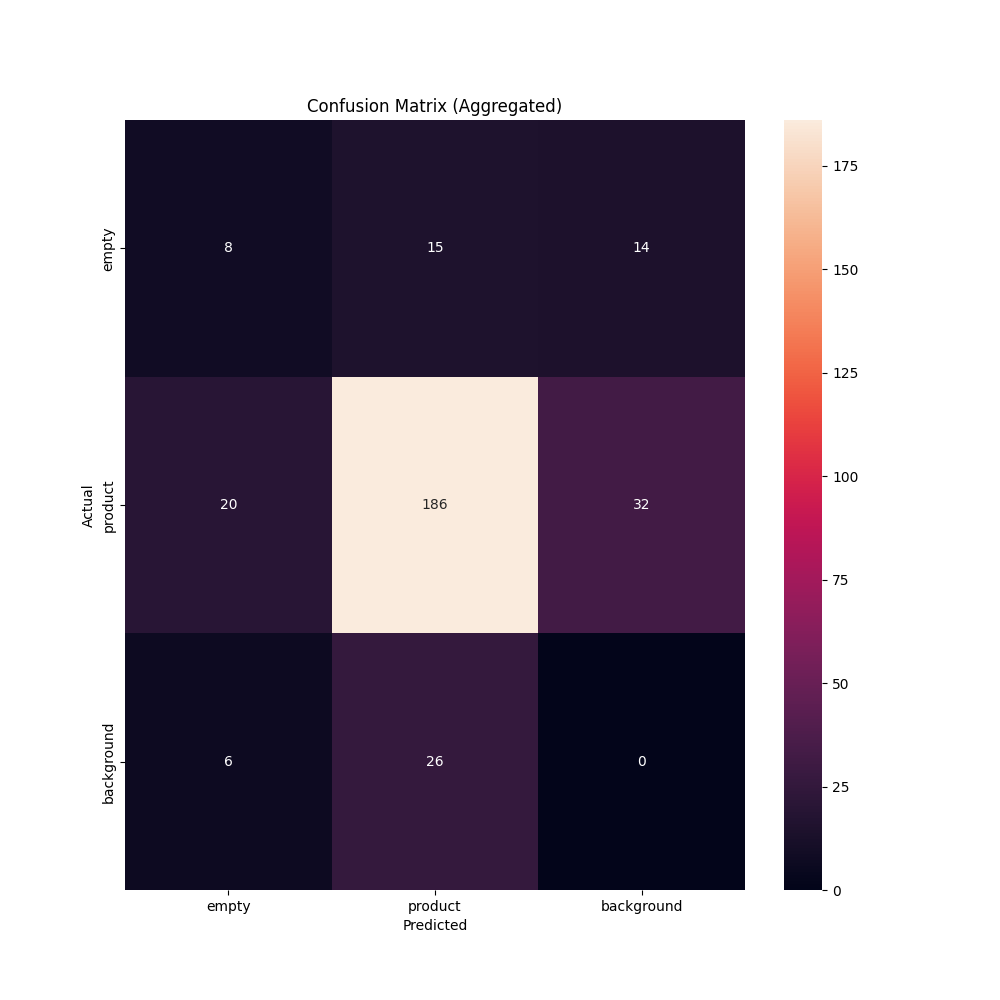
We can use this confusion matrix to understand true and false positive rates across our dataset and ascertain whether the values indicate our model is ready for production. From the matrix above, we can make determinations on whether the false positive rate is too high for any class. If it is, we can use that information to go back to our model and plan a strategy for improvement.

For instance, if a particular class has a high false positive rate, you may want to add more representative data for a given class then retrain your model. With a changed model, you can run your evaluation again to see how your changes impacted model performance.

Let’s open up one of the images in the output/images directory to visualize our model predictions:

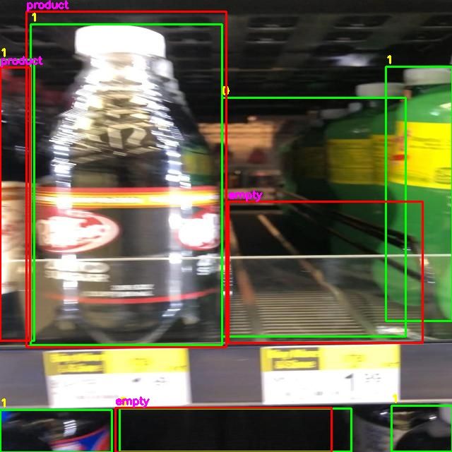
We can use these images to visualize how our model performs.

Ground truth – your annotations – are in green bounding boxes. Model predictions are in displayed inside red boxes.

From the above image, for example, we can see that our model has identified many of the spaces in the image, but it missed two on the bottom shelf. If you need to dive deep into model performance, these images can be a useful reference. For instance, if you see there are many false positives, you can review images to visualize instances of false positives.

Conclusion

In this guide, we have calculated precision, recall, and F1 metrics associated with an object detection model. We have also computed confusion matrices we can use to better understand how our model performs.

With this information, we can make decisions about the readiness of a model for production. If a model doesn’t perform as well as expected, you can use that information to make a plan about what to do next.

CVevals has a wide range of other features, too, such as allowing you to:

1. Compare different confidence levels to understand which one is best for use in production;
2. Evaluate the performance of various zero-shot models (Grounding DINO, CLIP, BLIP, and more) on your dataset, and;
3. Compare prompts for zero-shot models.

To find out more about the other features available in the library, check out the project README.