
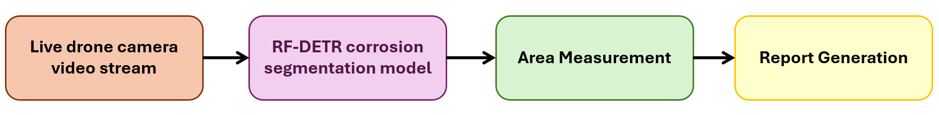
This tutorial builds a telecom tower corrosion inspection system using drone imagery, training an RF-DETR instance segmentation model to detect and segment corroded regions and wiring it into a Roboflow Workflow that measures corrosion area in pixels from a live drone video stream. Pixel measurements can be converted to real-world units using camera parameters, and the same pipeline can be extended to rank tower sites by severity, schedule accelerated inspections, and drive maintenance decisions across large tower networks.
Telecom towers are important utility infrastructure. They need to be inspected regularly to ensure structural integrity, verify that equipment is correctly installed, and catch defects before they lead to failures or service disruptions. Computer vision (CV) is the right technology for this kind of inspection work.
Mounted on a drone flying an inspection route around a tower, a camera captures detailed imagery of components that are difficult to document thoroughly from the ground. A CV model processes that imagery and flags specific conditions automatically, consistently, and across every frame. The result is a structured, visual record of the tower's condition that engineers can act on directly. There are several types of tower inspection where computer vision adds practical value:
- Corrosion detection: Identifying surface rust and coating degradation on structural steel, tower legs, bracing members, and hardware before it compromises load-bearing capacity.
- Missing or loose fasteners: Detecting absent or improperly installed bolts and nuts at joints and connection plates.
- Antenna misalignment: Flagging antennas that have physically shifted from their mounted position due to wind loading or improper installation.
- Cable damage: Identifying frayed, kinked, or improperly routed feeder cables and grounding conductors.
- Structural cracks: Detecting hairline or visible fractures in welds, members, and mounting hardware.
In this tutorial, we focus on corrosion detection and area measurement - one of the most common and consequential defects found on telecom towers. We will train an RF-DETR instance segmentation model to detect and segment corroded regions in drone imagery, build a Roboflow Workflow that measures the corrosion area in pixels from a live drone video stream, and show how to convert that pixel area to real-world units for reporting.
Output of the Telecom Tower Inspection System
So let's get started.
How to Build a Tower Inspection System with Roboflow
The following steps show how to build a telecom tower inspection system using Roboflow, that analyzes drone images to detect corrosion and measure its exact area in area_px. This helps move from simple detection to more accurate, data-driven maintenance decisions. Here's how the system works:
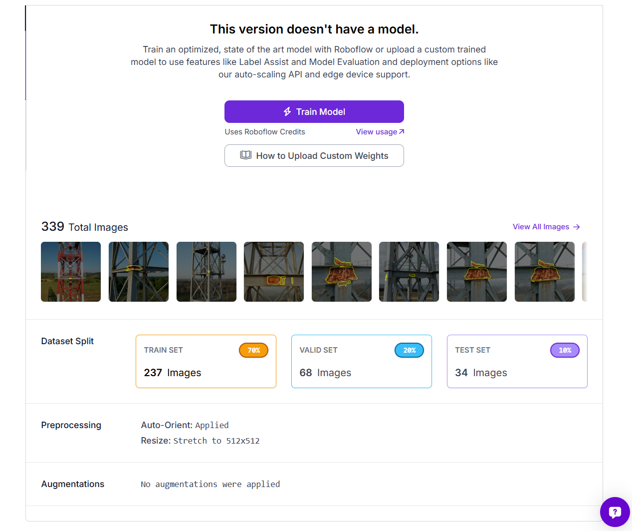
Step 1: Collect and annotate your dataset
Start by creating an Instance Segmentation project in Roboflow. This project type is important because we want to label the exact corrosion region as a mask, not just draw a box around it.
Upload and prepare images
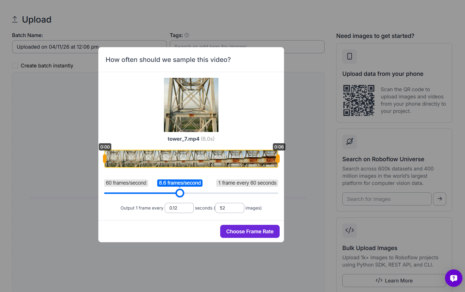
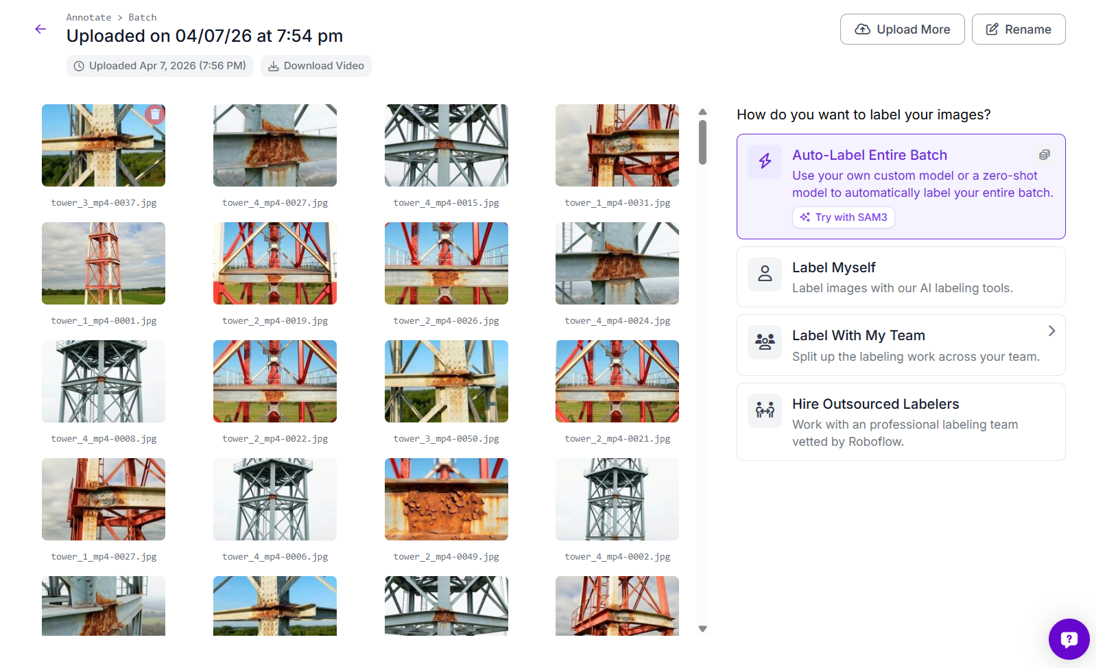
Upload your drone inspection video or images into Roboflow. If you are starting from video, you can use Roboflow’s frame extraction tool to pull frames at regular intervals. For this project, frames were taken from drone videos of telecom towers and uploaded as batches into Roboflow. The uploaded images included both full tower views and close-up shots of structural joints, bracing sections, and corroded members.
Over time, it is a good idea to expand the dataset with more variation. Try to include different tower angles, lighting conditions, corrosion patterns, and structural sections. This helps the model perform better on real inspection footage.
Use Auto Label with SAM 3
Since this is an instance segmentation task, each corrosion region needs a polygon mask. Drawing all of these by hand takes time, so Roboflow’s Auto Label feature makes the process much faster. Open the uploaded batch in Annotate and choose Auto-Label Entire Batch.
Select SAM 3 (Polygons) as the labeling model and create the class corrosion.
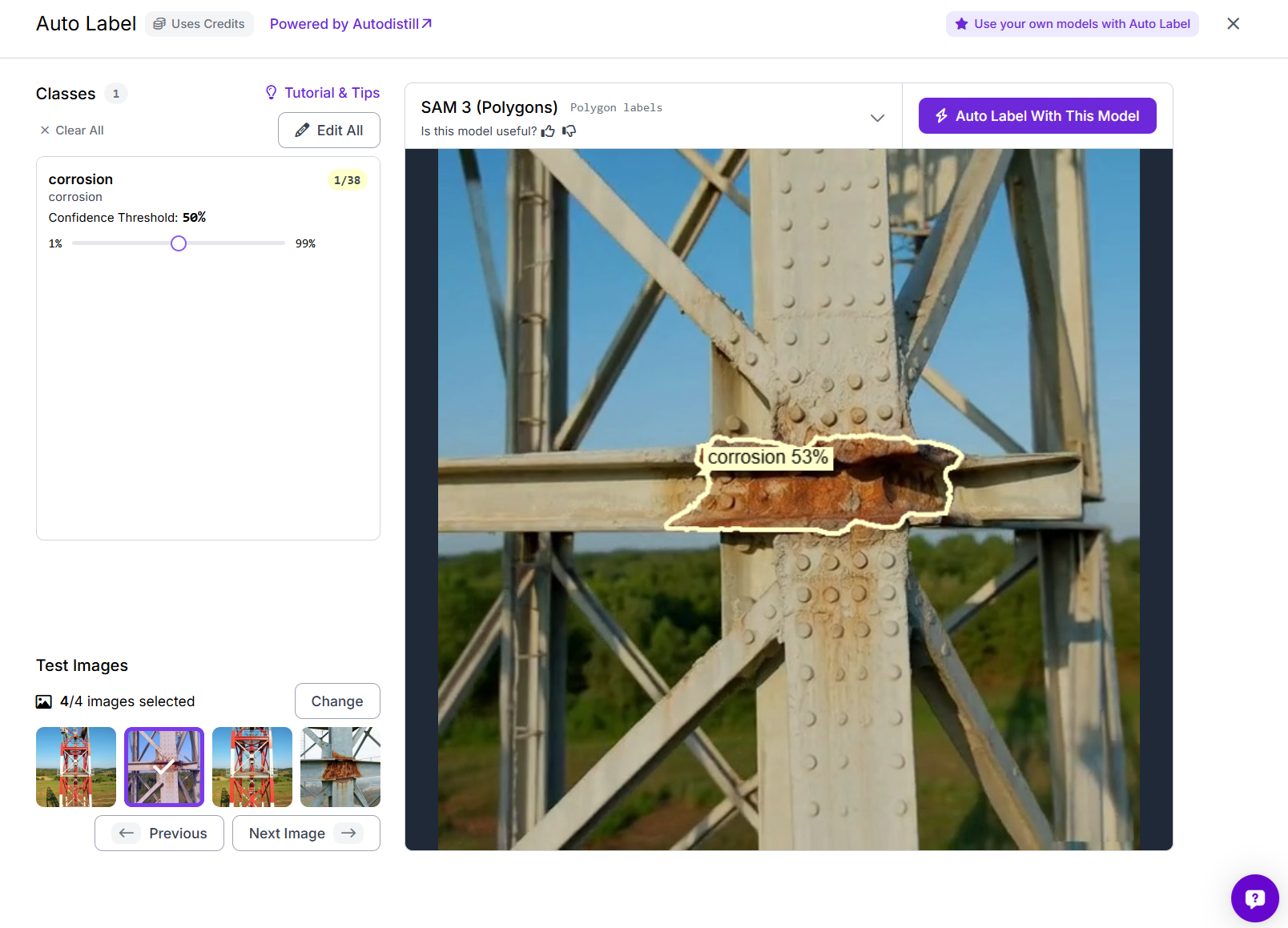
Roboflow lets you test the setup first on a few sample images, which is useful for checking whether the generated masks are following the corroded regions properly. Once the preview looks good, start the full auto-label job.
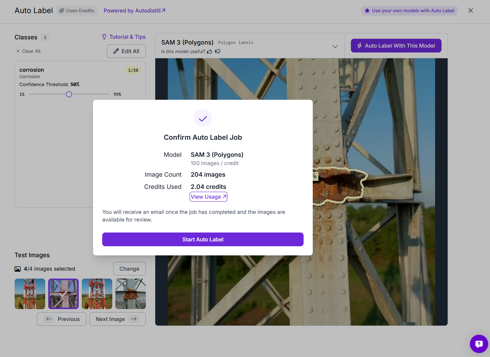
In this project, SAM 3 was used to label the batch automatically, generating polygon masks for the corrosion regions across all images.
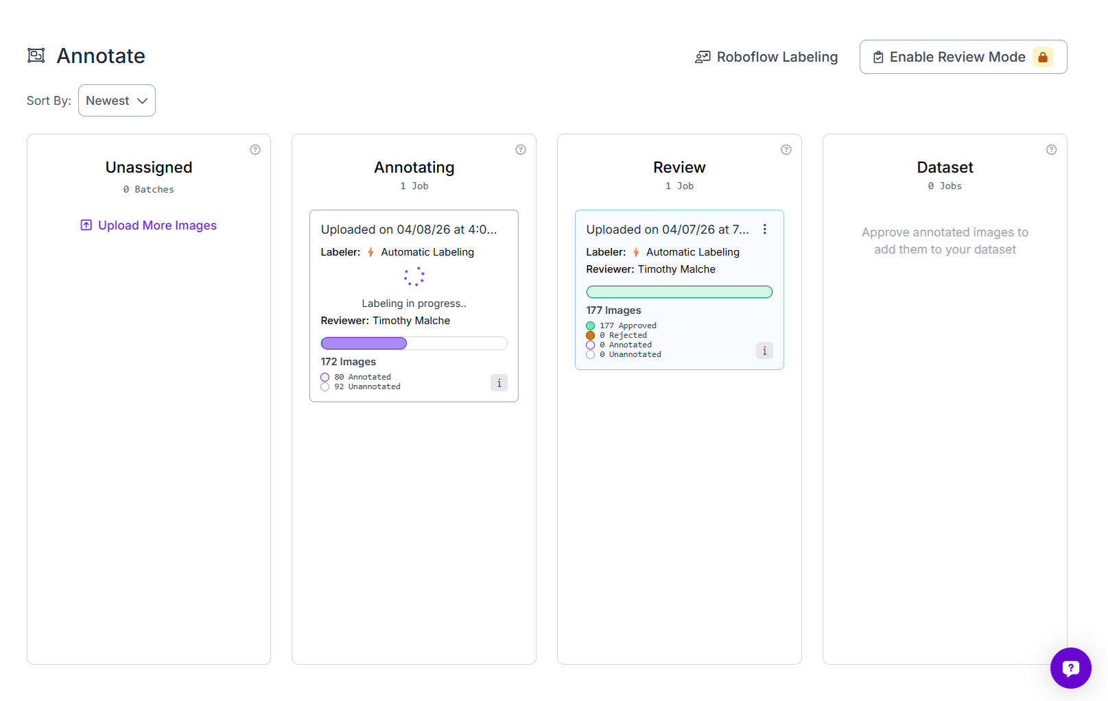
Review and approve annotations
After auto-labeling finishes, the batch moves into the Review stage.
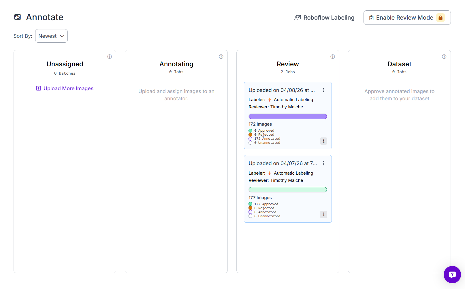
At this point, go through the images and check the generated masks carefully. Approve the good annotations and fix or reject the ones that are not accurate enough.
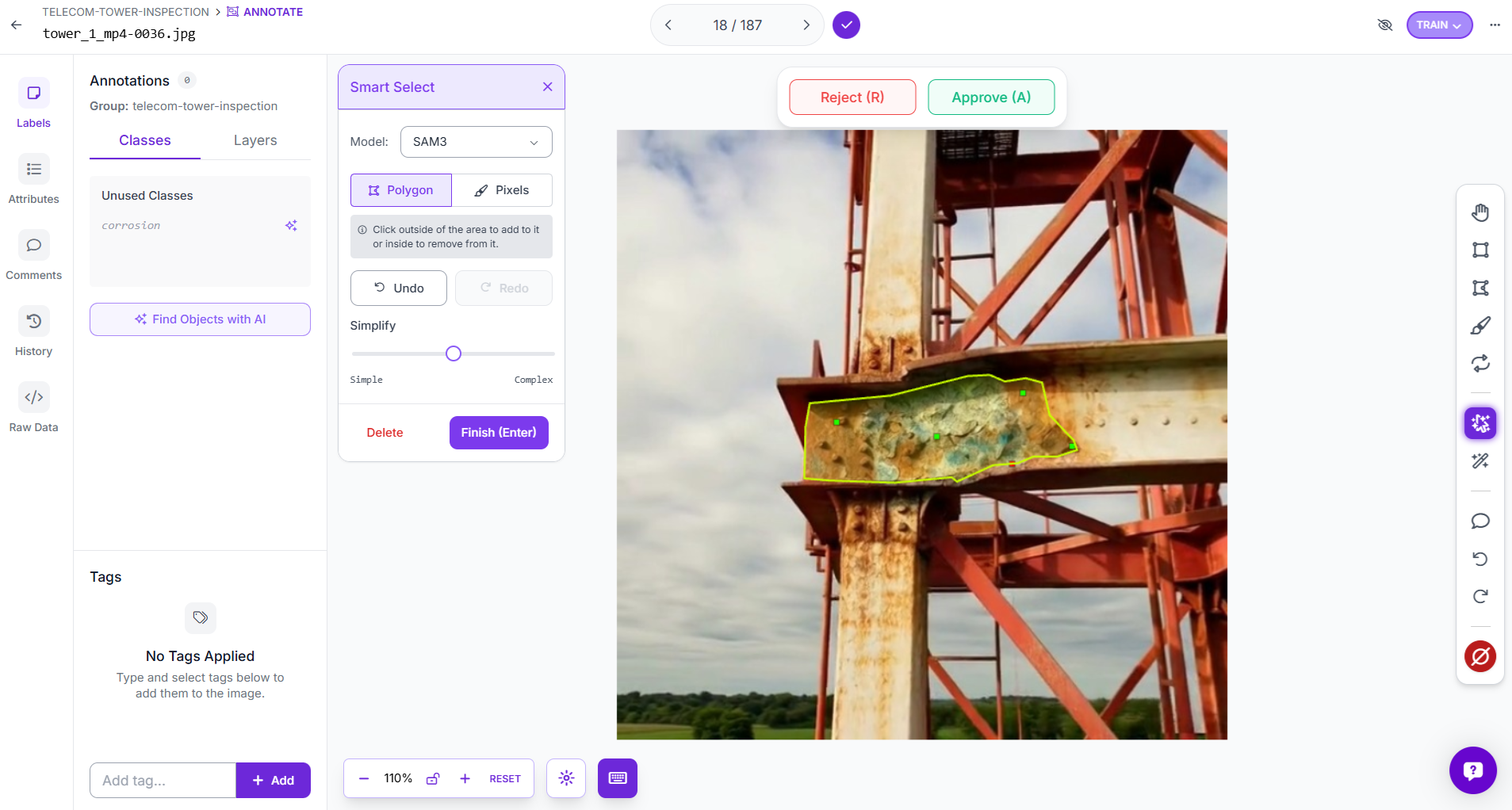
In this project, the review stage was used to verify that the corrosion masks matched the rusted regions closely before approving them into the dataset. This step is important because better labels usually lead to a better model.
Generate a dataset version
Once the annotations are ready, generate a new dataset version in Roboflow. Use these settings. You can apply preprocessing and augmentation. These augmentations help the model handle real inspection conditions, especially because corrosion can look different depending on lighting, paint condition, and metal surface appearance. After that, generate the dataset version for training.
Step 2: Train an RF-DETR Instance Segmentation Model
Navigate to your dataset version and click Train Model. Under Select Architecture, choose Roboflow RF-DETR. Set the Model Size to Small.
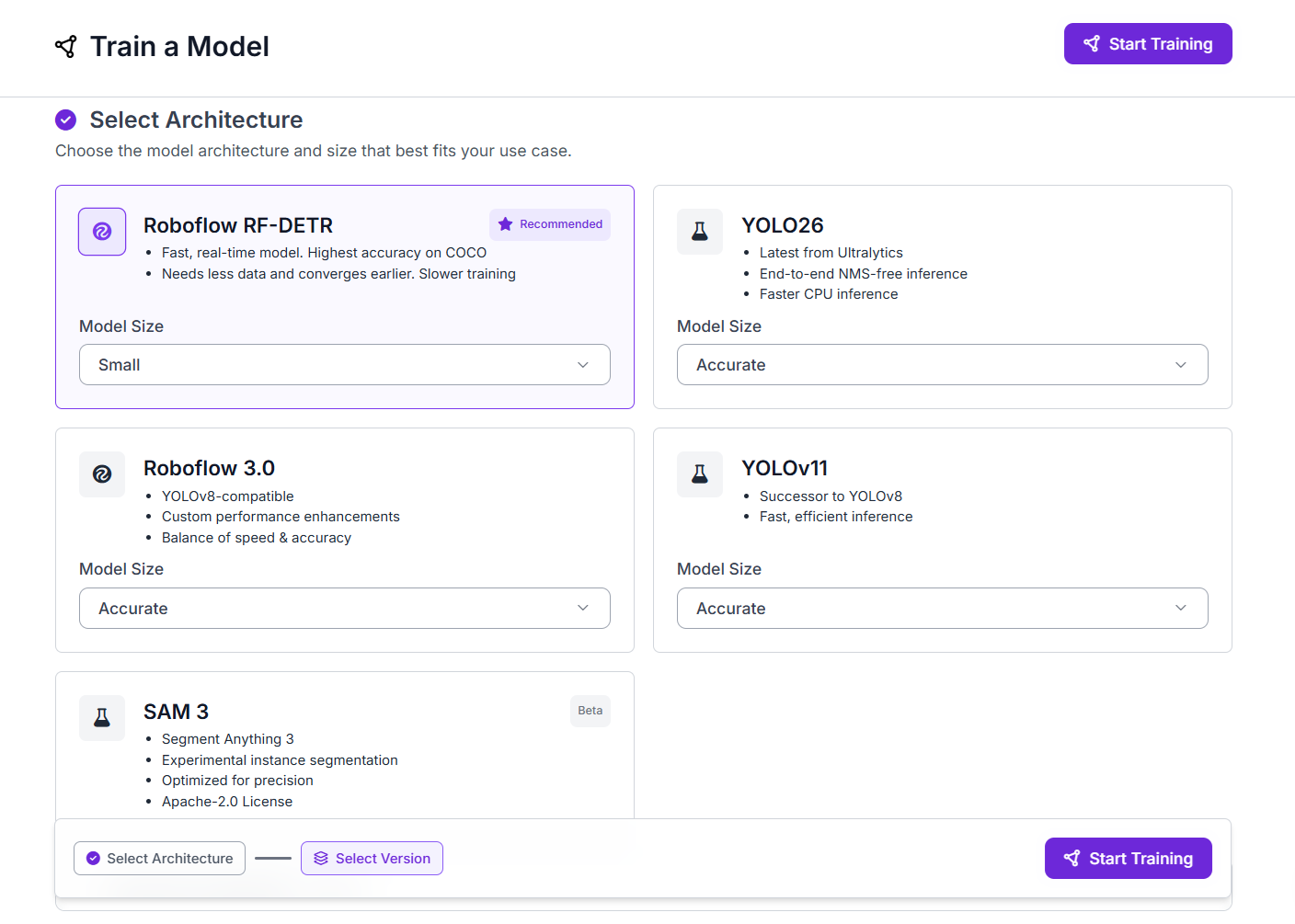
Click Start Training. Training runs on Roboflow's GPU infrastructure. No GPU setup, no training code, no infrastructure configuration required. You will receive an email when training is complete. Once done, the trained model appears in your Models tab.
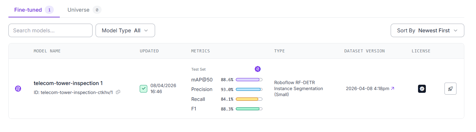
For this project, the trained model telecom-tower-inspection-ctkhv/1 produced the following results on the test set:
The model is hosted on Roboflow and ready to use via its model ID telecom-tower-inspection-ctkhv/1.
Step 3: Build the Corrosion Inspection Workflow
Now we will build the workflow. In your Roboflow dashboard, click Workflows in the left sidebar, then Create Workflow > Build My Own. The workflow is built in four blocks after the Image Input:
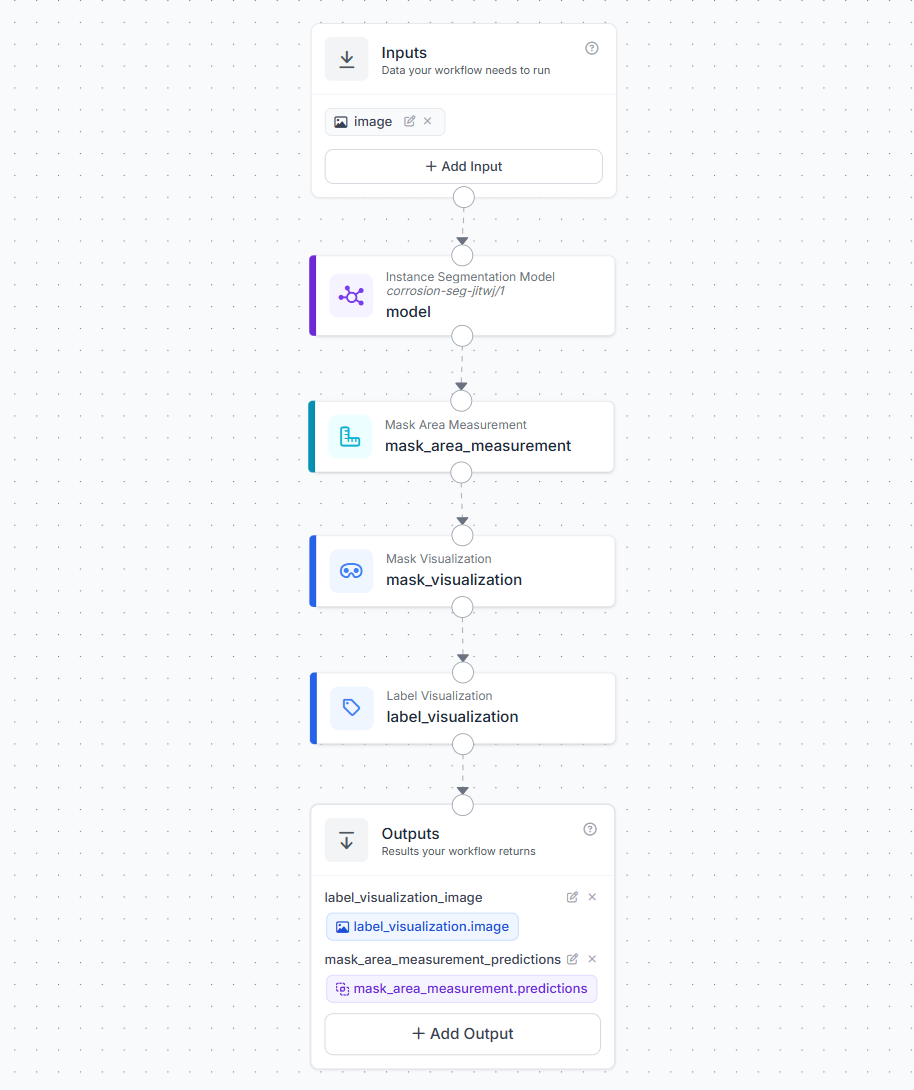
Block 1: Image Input
This is where your image or video frame enters the workflow.
Block 2: Instance Segmentation Model
- Connect to the image input
- Select your trained RF-DETR corrosion model (
telecom-tower-inspection-ctkhv/1) - Confidence threshold: 0.45
This block runs the RF-DETR model on every frame and returns segmentation masks, bounding boxes, class labels, and confidence scores for every detected corrosion instance.
Block 3: Mask Area Measurement
Add a Mask Area Measurement block.
- Predictions: Connect to the Instance Segmentation Model output (
model.predictions) - Pixels Per Unit: Leave at
1(default)
This is the core measurement block. For instance segmentation inputs, it counts the non-zero pixels in each mask using cv2.countNonZero. This correctly handles masks with holes. Hole pixels are zero and are excluded from the count. It attaches two values to each detection:
area_px- the corrosion area in square pixelsarea_converted- the area in real-world units (whenpixels_per_unitis 1, this equalsarea_px)
Block 4: Mask Visualization
- Image: Connect to the input image
- Predictions: Connect to the Mask Area Measurement output
This renders the segmentation mask polygons as colored overlays on the image.
Block 5: Label Visualization
Add a Label Visualization block.
- Input Image: Connect to the Mask Visualization output (
mask_visualization.image) - Predictions: Connect to the Mask Area Measurement output (
mask_area_measurement.predictions) - Text: Select "Area (mask)" from the dropdown
The Area (mask) text option pulls the area_px value from the Mask Area Measurement output and renders it as a label on each detected corrosion instance in the image. This is what gives you the live area reading overlaid on the drone stream.
Configure Outputs
In the Outputs section, add two outputs:
| Output Name | Source |
|---|---|
label_visualization_image | label_visualization.image |
mask_area_measurement_predictions | mask_area_measurement.predictions |
The first output is the annotated frame you display to the operator. The second is the structured prediction data, each detection has its class, confidence, bounding box, mask polygon, area_px, and area_converted which feeds your inspection report.
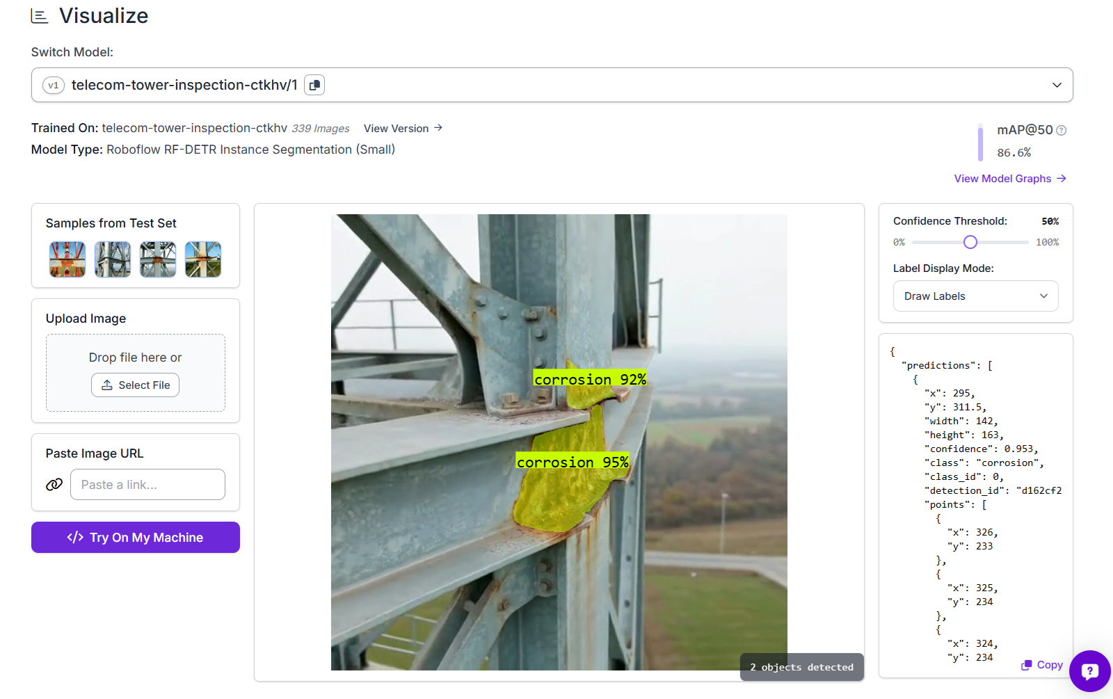
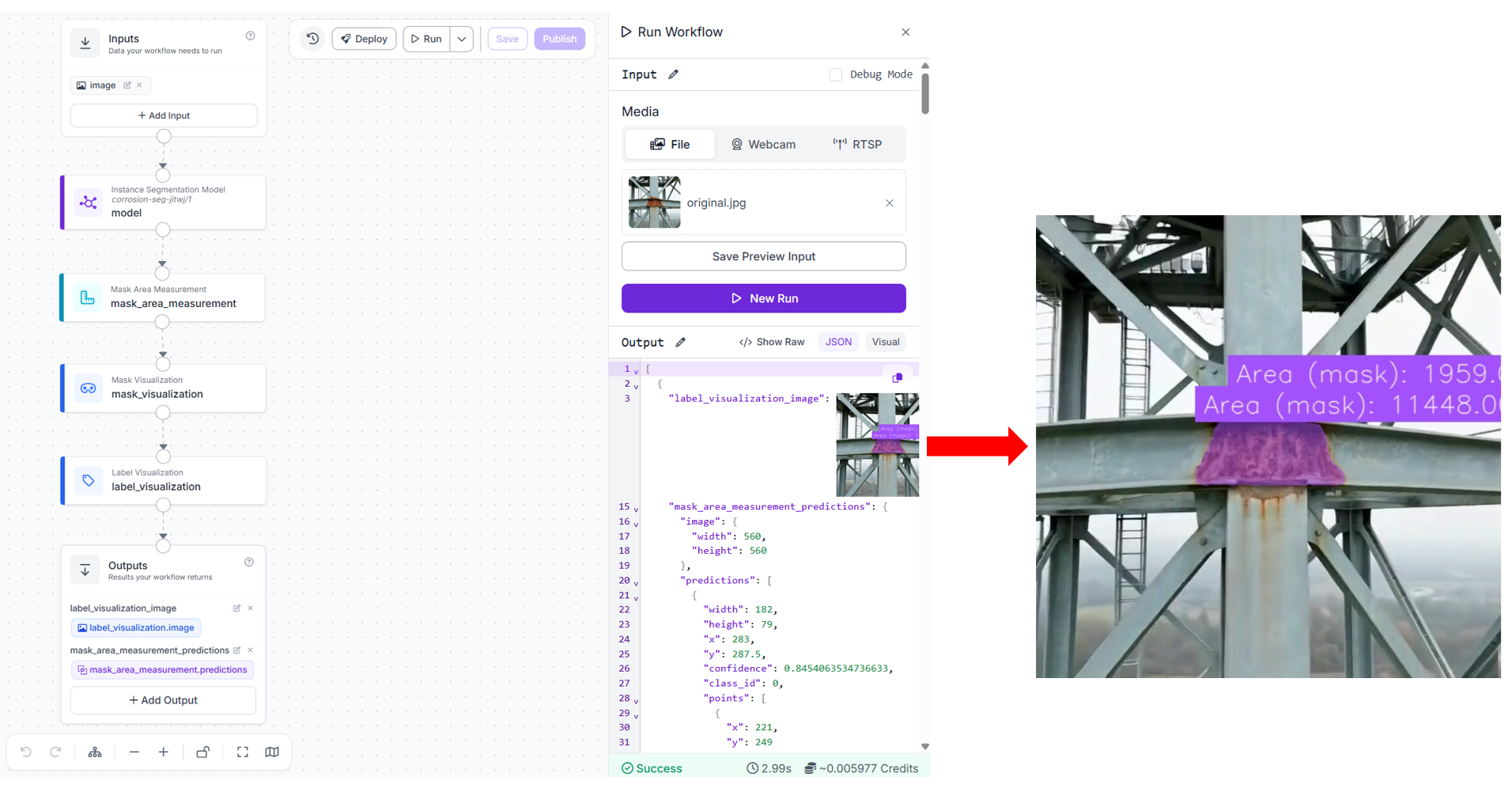
When you run the workflow (uploading an image), you should see output similar to following.
Step 4: Deploy for Live Drone Stream Processing
Install the inference SDK:
pip install -U inference-sdkThe deployment uses Roboflow's inference SDK WebRTC streaming pipeline. Instead of pulling frames in a manual loop, InferenceHTTPClient opens a persistent WebRTC session with the RTSP source. Two separate callbacks handle the two output channels: on_frame receives the annotated video frames and displays them live, and on_data receives the structured prediction data per frame via a datachannel. Here's the code for tower_inspect.py
import cv2
import json
from datetime import datetime
from inference_sdk import InferenceHTTPClient
from inference_sdk.webrtc import RTSPSource, StreamConfig, VideoMetadata

SITE_ID    = "SITE-4271"
SITE_NAME  = "Tower 4 - Northern Grid Sector B"
INSPECTOR  = "Timothy M."

client = InferenceHTTPClient.init(
    api_url="https://serverless.roboflow.com",
    api_key="YOUR_ROBOFLOW_API_KEY"
)

# Replace with your drone's RTSP stream URL.
source = RTSPSource("rtsp://YOUR_DRONE_RTSP_URL")

config = StreamConfig(
    stream_output=["label_visualization_image"],
    data_output=["mask_area_measurement_predictions"],
    processing_timeout=3600,
    requested_plan="webrtc-gpu-medium",
    requested_region="us"
)

session = client.webrtc.stream(
    source=source,
    workflow="telecom-tower-inspection",
    workspace="tim-4ijf0",
    image_input="image",
    config=config
)

detection_log = []

@session.on_frame
def show_frame(frame, metadata):
    cv2.imshow("Tower Inspection - Live", frame)
    if cv2.waitKey(1) & 0xFF == ord("q"):
        session.close()

@session.on_data()
def on_data(data: dict, metadata: VideoMetadata):
    preds = data.get(
        "mask_area_measurement_predictions", {}
    ).get("predictions", [])

    for p in preds:
        area_px    = p.get("area_px", 0)
        confidence = p.get("confidence", 0)

        detection_log.append({
            "frame_id":   metadata.frame_id,
            "confidence": round(confidence, 3),
            "area_px":    area_px,
        })

        print(
            f"[frame {metadata.frame_id}] "
            f"corrosion | confidence={confidence:.2f} | area_px={area_px}"
        )

session.run()

def generate_report(site_id, site_name, inspector, detections):

    # Keep only the single highest-confidence detection
    # across the entire flight — one entry per corrosion instance
    peak = max(detections, key=lambda d: d["area_px"]) if detections else None

    report = {
        "site_id":             site_id,
        "site_name":           site_name,
        "inspector":           inspector,
        "inspection_date":     datetime.now().strftime("%Y-%m-%d"),
        "inspection_time":     datetime.now().strftime("%H:%M:%S"),
        "corrosion_detected":  bool(peak),
        "peak_area_px":        peak["area_px"] if peak else 0,
        "peak_confidence":     peak["confidence"] if peak else 0,
        "peak_frame_id":       peak["frame_id"] if peak else None,
        "frame_detections":    detections
    }

    filename = f"inspection_report_{site_id}_{datetime.now().strftime('%Y%m%d')}.json"
    with open(filename, "w") as f:
        json.dump(report, f, indent=2)

    print(f"\n{'='*50}")
    print(f"INSPECTION REPORT - {site_id}")
    print(f"{'='*50}")
    print(f"Site:              {site_name}")
    print(f"Inspector:         {inspector}")
    print(f"Date:              {report['inspection_date']}")
    print(f"Corrosion detected:{report['corrosion_detected']}")
    print(f"Peak area:         {report['peak_area_px']} px")
    print(f"Peak confidence:   {report['peak_confidence']}")
    print(f"Report saved:      {filename}")

generate_report(SITE_ID, SITE_NAME, INSPECTOR, detection_log)
RTSPSource wraps the drone's live RTSP stream as the WebRTC input. Every frame from the stream is forwarded to the Roboflow cloud worker running your Workflow. StreamConfig controls what comes back. stream_output specifies which Workflow outputs are returned as a video stream, here label_visualization_image, the annotated frame from your Label Visualization block. data_output specifies which outputs are returned as structured data per frame, here mask_area_measurement_predictions, which contains every corrosion detection with its area_px. @session.on_frame fires for every annotated video frame received. It displays the frame in an OpenCV window. Pressing q closes the session cleanly.
@session.on_data() fires for every frame's prediction data. The data dict contains the mask_area_measurement_predictions output. Each prediction in predictions includes the class, confidence, bounding box, segmentation mask polygon, area_px, and area_converted. The metadata.frame_id links the prediction data back to the corresponding video frame. session.run() blocks until the session is closed (by pressing q) or the processing_timeout is reached. When the drone flies past a corroded section of a tower leg:
[frame 311] corrosion | confidence=0.84 | area_px=4102
[frame 312] corrosion | confidence=0.87 | area_px=4821
[frame 313] corrosion | confidence=0.89 | area_px=4934
[frame 314] corrosion | confidence=0.91 | area_px=5102
[frame 315] corrosion | confidence=0.90 | area_px=5089
The area_px values are stable across consecutive frames as the drone holds position, confirming a genuine corrosion instance rather than a single-frame false positive. The annotated live window simultaneously shows the segmentation mask with the area_px label rendered on the corrosion region.
Once the session ends, the report is generated automatically and saved as a JSON file. The peak detection, the single frame with the highest area_px across the entire flight, is used to represent the corrosion instance, avoiding inflated counts from the same patch being detected across multiple consecutive frames.
{
  "site_id": "SITE-4271",
  "site_name": "Tower 4 — Northern Grid Sector B",
  "inspector": "Timothy M.",
  "inspection_date": "2026-04-09",
  "inspection_time": "10:23:44",
  "corrosion_detected": true,
  "peak_area_px": 5102,
  "peak_confidence": 0.91,
  "peak_frame_id": 314,
  "frame_detections": [
    { "frame_id": 311, "confidence": 0.84, "area_px": 4102 },
    { "frame_id": 312, "confidence": 0.87, "area_px": 4821 },
    { "frame_id": 313, "confidence": 0.89, "area_px": 4934 },
    { "frame_id": 314, "confidence": 0.91, "area_px": 5102 },
    { "frame_id": 315, "confidence": 0.90, "area_px": 5089 }
  ]
}
And the terminal summary printed at the end of the flight:
==================================================
INSPECTION REPORT — SITE-4271
==================================================
Site:              Tower 4 — Northern Grid Sector B
Inspector:         Timothy M.
Date:              2026-04-09
Corrosion detected:True
Peak area:         5102 px
Peak confidence:   0.91
Report saved:      inspection_report_SITE-4271_20260409.json
You may also try this example on captured video file by importing the required libraries,
from inference_sdk.webrtc import VideoFileSource, StreamConfig, VideoMetadataand using the video source,
source = VideoFileSource("tower_5.mp4", realtime_processing=False)Step 5: Converting area_px to Real-World Units
In our workflow, the Mask Area Measurement block outputs area_px, the count of non-zero pixels inside the segmentation mask, computed using cv2.countNonZero. This correctly handles masks with holes, since hole pixels are zero and are excluded from the count. Alongside area_px, the block also computes area_converted using this formula:
area_converted = area_px / (pixels_per_unit ** 2)When pixels_per_unit is left at its default of 1.0, area_converted equals area_px. To get a real-world area, you provide a pixels_per_unit calibration value, the number of pixels that correspond to one unit of real-world length (e.g., pixels per cm) and the block handles the rest.
pixels_per_unit value you calibrate is only accurate at the specific distance from which you measured it. To keep real-world area values consistent, you can use a pre-programmed waypoint route, manually fly at a fixed standoff distance, or place a reference object of known size on the tower structure to recalibrate from any frame where it is visible.Extending the System
Once the base workflow is working, you can extend it to solve more inspection tasks. The same pipeline can be used for more defect types, long-term tracking, and site-level maintenance planning.
- Multi-class defect detection: The same workflow can be extended to inspect other tower defects such as corrosion, cracks, missing bolts, damaged cables, and antenna issues. In practice, you can combine both instance segmentation and object detection models in the same workflow. Segmentation is useful for defects where shape and area matter, such as corrosion and cracks, while object detection works well for defects like missing bolts or antenna misalignment where location is more important than mask area. This makes the system more flexible for real inspection use cases.
- Trend tracking across inspection cycles: Store the
area_pxvalues from each inspection cycle in a database keyed by site ID, tower zone, and inspection date. Query for corrosion instances wherearea_pxhas grown significantly between consecutive inspections. A corroded section that doubles in area between two annual inspections is flagged for accelerated inspection scheduling, even if its absolute size is still within acceptable limits. - Automatic severity scoring: You can add a post-processing step after inference to assign a severity score for each tower site. This score can consider the total corrosion area, the number of corrosion spots, the type of corrosion observed such as surface rust, coating loss, or deeper corrosion, and where it appears on the tower. Based on this score, sites can be ranked so maintenance teams can focus first on the most critical towers.
This approach turns inspection from simple visual checking into a structured, data-driven process, helping teams make faster and more informed maintenance decisions across large tower networks.
Conclusion: Inspecting Telecom Towers with Computer Vision
Computer vision is a practical addition to telecom tower inspection workflows, giving teams better visibility into structural conditions and a more structured way to document and track defects over time. To build your own telecom tower inspection system, create a free Roboflow account and get started with the steps above, or connect with a computer vision expert to discuss your specific use case.
Cite this Post
Use the following entry to cite this post in your research:
Timothy M. (Apr 13, 2026). Inspecting Telecom Towers with Computer Vision. Roboflow Blog: https://blog.roboflow.com/inspecting-telecom-towers-with-computer-vision/