

mAP@0.5 evaluates detection at a single IoU threshold of 0.50, while mAP@0.5:0.95 evaluates it across ten thresholds from 0.50 to 0.95, providing a stricter measure of a model’s detection and localization accuracy. This guide covers what these metrics mean, how they are calculated, and when to use them.
When evaluating an object detection model, you will often see metrics such as mAP@0.5 and mAP@0.5:0.95. Both measure how well a model detects objects, but they evaluate bounding box quality at different levels of strictness.
The key difference is simple: mAP@0.5 evaluates predictions at a single IoU threshold of 0.50, while mAP@0.5:0.95 evaluates predictions across ten IoU thresholds from 0.50 to 0.95 and averages the results.
In this guide, we’ll break down the concepts behind mAP and IoU thresholds step by step:
- First, we’ll understand Precision and Recall.
- Then, we’ll look at Confidence Scores.
- Next, we’ll use these concepts to calculate Average Precision (AP).
- Then, we’ll see how AP is used to calculate Mean Average Precision (mAP).
- Finally, we’ll introduce IoU thresholds and understand the difference between mAP@0.5 and mAP@0.5:0.95.
By the end, you’ll understand how these metrics are calculated, what they tell you about an object detection model, and when to use mAP@0.5 versus mAP@0.5:0.95.
Understanding Precision and Recall
What Is Precision?
Precision measures how many of the model's positive predictions for a specific object class are correct. In object detection, a positive prediction means that the model has detected an object and assigned it to the target class.
High precision means that the model's predictions for that class are usually correct, with relatively few false positives. A false positive (FP) occurs when the model predicts an object as belonging to a class, but the prediction does not correctly match a ground-truth object of that class.
Low precision means that the model frequently makes incorrect detections for that class, resulting in more false positives.
Precision is especially important when false positives are costly. For example, in a defect detection system, a false positive could cause a non-defective product to be incorrectly rejected.
What Is Recall?
Recall measures how many of the actual objects belonging to a specific class the model successfully detects. In object detection, an actual positive case means that an object of the target class is present in the ground-truth annotations.
High recall means that the model detects most of the objects of a class that are actually present. Low recall means that the model misses many objects of that class, resulting in more false negatives.
A false negative (FN) occurs when an object belonging to a specific class is present in the ground truth, but the model fails to detect it correctly.
Recall is especially important when false negatives are costly. For example, in defect detection, missing a defective product could allow a faulty item to reach customers.
How Are Precision and Recall Calculated?
Precision and Recall are calculated using True Positives (TP), False Positives (FP), and False Negatives (FN). In object detection, these values are class-specific, meaning each object class has its own TP, FP, and FN counts. As a result, Precision and Recall are also class-specific.
These values can be determined by comparing the model's predictions with the ground-truth annotations and organizing the results in a confusion matrix, as shown below.
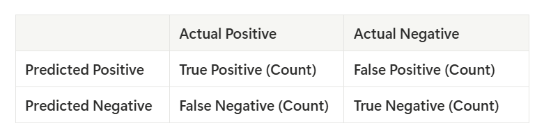
Where:
- When a model correctly identifies an object as belonging to the positive class, it is a True Positive (TP).
- When the model predicts an object or class that is not actually present, it is a False Positive (FP).
- Similarly, a False Negative (FN) occurs when the model fails to detect an object that is actually present
- While a True Negative (TN) occurs when the model correctly identifies the absence of an object.
You can then use the formula below to calculate the Precision:

You can then use the formula below to calculate the Recall:

In the above formulas, TP, FP, and FN represent the total number of True Positives, False Positives, and False Negatives, respectively for a specific class. True Negatives (TN) are generally not required to calculate Precision and Recall in object detection.
Understanding Confidence Scores
What Is a Confidence Score?
A confidence score indicates how confident an object detection model is in a prediction, including the predicted object class and its location.
Based on the confidence score, the researcher, developer, or engineer sets a confidence threshold to determine which predictions are accepted as detections and which are rejected.
For example, an object detection model might return a prediction in JSON format like the following:
{
  "class": "car",
  "confidence": 0.92,
  "bounding_box": {
    "x": 120,
    "y": 80,
    "width": 200,
    "height": 150
  }
}
Example of an predicted car object
How Does the Confidence Threshold Affect Precision and Recall?
Changing the confidence threshold changes which predictions are accepted as detections, which in turn affects the model's Precision and Recall for a class.
A higher threshold typically results in fewer, more confident detections, while a lower threshold allows more predictions to be accepted but may also introduce more false positives.
For example, suppose an object detection model produces four predictions for the car class with confidence scores of 0.95, 0.85, 0.65, and 0.40.
If the confidence threshold is set to 0.80, only the predictions with confidence scores of 0.95 and 0.85 are accepted. If the threshold is lowered to 0.50, the prediction with a confidence score of 0.65 is also accepted.
In general:
- Higher confidence threshold -> generally higher precision, lower recall: Only the most confident predictions are accepted as detections. This can reduce false positives but may also cause the model to miss some actual objects.
- Lower confidence threshold -> generally lower precision, higher recall: More predictions are accepted as detections, which can help detect more actual objects but may also increase false positives.
Therefore, there is usually a trade-off between Precision and Recall when selecting a confidence threshold. The best threshold depends on the application and whether it is more important to minimize false positives or minimize missed detections.
Understanding Average Precision (AP)
What Is a Precision-Recall Curve?
As explained above, changing the confidence threshold changes the model's Precision and Recall for a class. By evaluating the model at different confidence thresholds, we can plot a Precision-Recall (PR) curve to visualize the relationship between Precision and Recall.
- Y-axis: Precision
- X-axis: Recall

What Is Average Precision?
Average Precision (AP) summarizes the Precision-Recall curve for an individual class into a single value by measuring the area under the curve (AUC).
A higher AP indicates that the model maintains higher precision across different levels of recall, indicating better overall detection performance for that class.
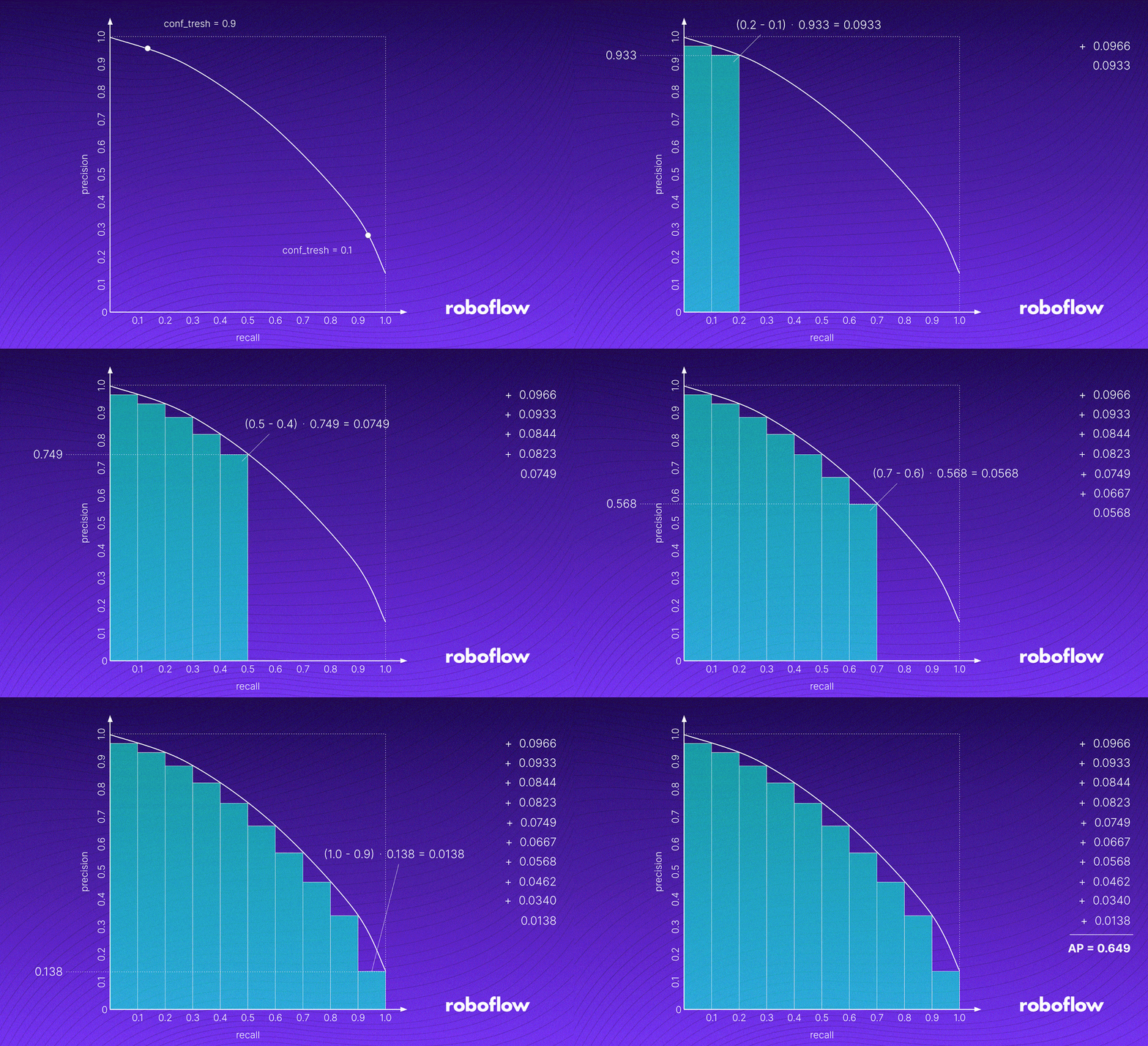
AP can be approximated by summing the areas of small rectangles under the Precision-Recall curve. Mathematically, this can be expressed using a discrete Riemann sum:

Where:
- P(Ri) is the precision at the right endpoint of the i-th recall interval.
- Ri − Ri−1 is the width of the recall interval.
- n is the total number of recall intervals.
Instead of selecting a single confidence threshold and reporting, "The model has 75% precision and 80% recall for this class," AP evaluates the model across multiple confidence thresholds, considers the resulting Precision-Recall relationship, and summarizes its overall performance for that class in a single value.
Understanding Mean Average Precision (mAP)
What Is mAP?
Mean Average Precision (mAP) summarizes an object detection model's performance across all object classes by averaging their Average Precision (AP) values. The resulting score ranges from 0 to 1 and is often reported as a percentage.
In other words, mAP is the mean of the Average Precision (AP) values across all detection classes in an object detection model.
How Is mAP Calculated?

Where:
- N is the total number of classes.
- APi is the Average Precision for class i.
For example, consider an object detection model capable of detecting various types of vehicles, with:

This means the model achieves an AP of 0.82 for the car class. Once the AP has been calculated for every class, we calculate mAP by taking the mean of the AP values across all classes:

where (N) is the total number of detection classes.
Understanding IoU and IoU Thresholds
What Is Intersection over Union (IoU)?
IoU (Intersection over Union) measures how much a predicted bounding box overlaps with the ground-truth bounding box.
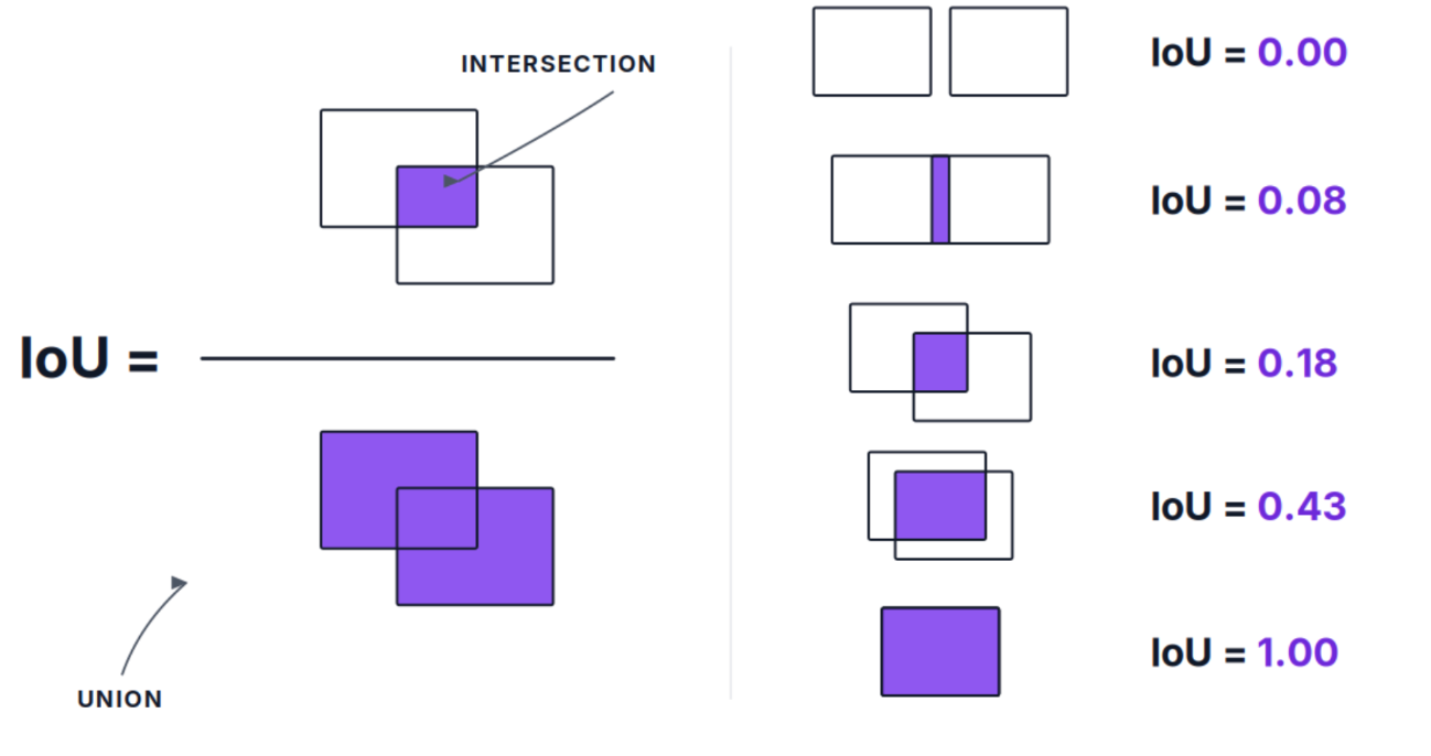
The formula is:

It is commonly used to evaluate the localization accuracy of an object detection model. Localization refers to the model's ability to accurately determine where an object is located in an image by placing a bounding box around it.
A model can correctly identify an object but still have poor localization if its predicted bounding box does not closely align with the actual object.
The examples below demonstrate ground-truth bounding boxes (green) and predicted bounding boxes (other colors), along with their corresponding IoU values.

What Is an IoU Threshold?
The IoU threshold is the minimum IoU value required for a prediction to be considered a correct detection (True Positive).
A lower IoU threshold is more forgiving, while a higher IoU threshold requires the predicted box to align more closely with the ground-truth box.
For example, if the IoU threshold is 0.4:
- IoU ≥ 0.4 → prediction is considered a True Positive
- IoU < 0.4 → prediction is considered a False Positive
What Is mAP@0.5?
mAP@0.5 refers to calculating mean Average Precision (mAP) using a single IoU threshold of 0.5.
At an IoU threshold of 0.5, a predicted bounding box must have an IoU of at least 0.5 with the corresponding ground-truth bounding box to be considered a True Positive (TP).
The IoU threshold determines whether a prediction is considered a TP or FP. Therefore, changing the IoU threshold can change the number of TPs, FPs, and FNs, which in turn affects Precision, Recall, AP, and ultimately mAP.
Earlier, when we calculated AP and mAP, we did not explicitly specify an IoU threshold. The threshold could be 0.3, 0.4, 0.5, or any other value between 0 and 1. At that stage, we assumed that the TPs, FPs, and FNs had already been determined based on a chosen IoU threshold.
To indicate the IoU threshold used to calculate mAP, the threshold is specified after the “@” symbol. For example:
- mAP@0.5 uses an IoU threshold of 0.50.
- mAP@0.75 uses an IoU threshold of 0.75.
mAP@0.5 is also commonly denoted as mAP50 or mAP@50.
How Is mAP@0.5 Calculated?
mAP@0.5 is calculated by first calculating AP for each class using a single IoU threshold of 0.50, then averaging the AP values across all classes.

Where:
- N is the total number of classes.
- APi@0.5 is the Average Precision for class i at an IoU threshold of 0.5.
For example, for a vehicle detection model the mAP@0.5 would be calculated as shown below:

What Does mAP@0.5 Tell You?
mAP@0.5 tells us “How well does the model detect objects when we require at least 50% overlap between the predicted and ground-truth bounding boxes?”
Because an IoU threshold of 0.5 is relatively forgiving, a prediction does not need to align extremely closely with the ground-truth bounding box to be considered correct.
This makes mAP@0.5 useful for evaluating a model's overall object detection performance when approximate bounding-box localization is sufficient.
What Is mAP@0.5:0.95?
mAP@0.5:0.95 is the mean of the mAP values calculated at 10 different IoU thresholds, ranging from 0.50 to 0.95 in increments of 0.05.
Unlike mAP@0.5, which evaluates the model using only a single IoU threshold of 0.50, mAP@0.5:0.95 evaluates the model across multiple IoU thresholds. This provides a stricter assessment of both object detection and bounding-box localization accuracy.
The 10 IoU thresholds are: 0.50, 0.55, 0.60, 0.65, 0.70, 0.75, 0.80, 0.85, 0.90, and 0.95.
mAP@0.5:0.95 is also commonly denoted as mAP50-95 or mAP@50:95.
How Is mAP@0.5:0.95 Calculated?
At each of the 10 IoU thresholds, mAP is calculated separately. The resulting 10 mAP values are then averaged to obtain the final mAP@0.5:0.95 score.

Equivalently,

Why Is mAP@0.5:0.95 Usually Lower Than mAP@0.5?
mAP@0.5:0.95 is usually lower than mAP@0.5 because it averages AP across increasingly strict IoU thresholds.
As the IoU threshold increases, fewer predictions meet the required overlap with the ground-truth boxes to be considered True Positives. Consequently, AP generally decreases at higher IoU thresholds because predictions that would have been considered correct at a lower threshold may no longer qualify as True Positives.
These lower AP values at stricter thresholds reduce the overall average, making mAP@0.5:0.95 a more demanding measure of both object detection performance and bounding-box localization accuracy.
When Should You Use mAP@0.5 vs. mAP@0.5:0.95?
The choice between these metrics depends on which aspect of object detection performance you want to evaluate.
When Should You Use mAP@0.5?
- You want a simple measure of detection performance.
- Approximate bounding box localization is sufficient.
- Your application prioritizes detecting objects over precise localization.
- You want to evaluate whether a model is making generally correct detections.
mAP@0.5 is useful for assessing whether a model can detect objects with reasonably accurate bounding boxes, but it does not provide a complete picture of localization quality. In simple terms, mAP@0.5 answers: “Can the model detect the object with a reasonably accurate bounding box?”
When Should You Use mAP@0.5:0.95?
- You want a more comprehensive evaluation of detection performance.
- Precise bounding box localization is important.
- You are comparing modern object detection models.
- You want to evaluate your model using the COCO evaluation protocol.
Because mAP@0.5:0.95 evaluates performance across multiple IoU thresholds from 0.50 to 0.95, it is generally a more informative metric for assessing overall object detection performance. In simple terms, mAP@0.5:0.95 answers: “Can the model detect the object and consistently localize it precisely?”
How to Get mAP Values from Roboflow Train
Roboflow Train is a model training platform by Roboflow that lets you train computer vision models on your annotated datasets without the need to manage complex training infrastructure or write training code. Learn how to train an object detection model.
Roboflow Train supports training computer vision models for tasks such as object detection, instance segmentation, semantic segmentation, classification, and keypoint detection.
With Roboflow Train, you can:
- Upload and version datasets
- Apply preprocessing and augmentations to entire datasets
- Train state-of-the-art models
- Evaluate model performance
- Deploy models for inference
When you train an object detection model using Roboflow Train, it reports key mAP metrics, including mAP@0.5, mAP@0.75, and mAP@0.5:0.95.
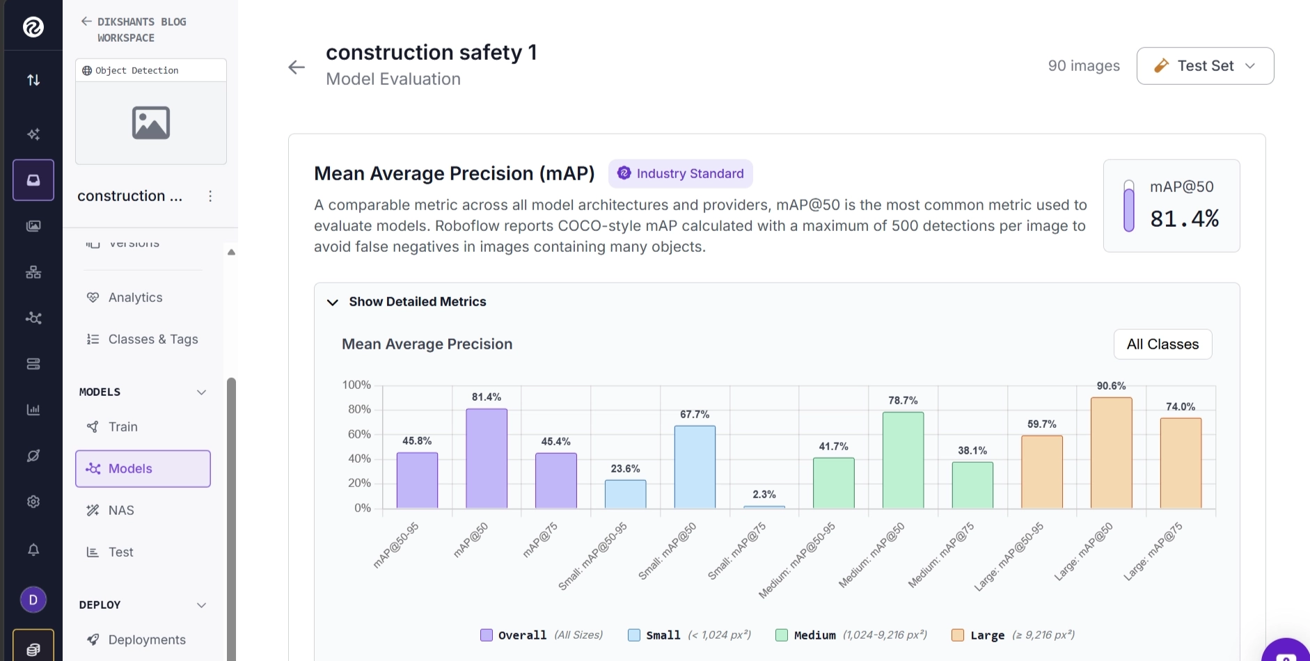
Roboflow provides mAP@0.5:0.95, mAP@0.5, and mAP@0.75 across All, Small, Medium, and Large object sizes to provide a more detailed evaluation of object detection performance.
In Roboflow, Small, Medium, and Large refer to the size of an object's ground-truth bounding box, measured by its area in pixels. These categories follow the COCO evaluation convention:
- Small: Bounding-box area is less than 1,024 pixels².
- Medium: Bounding-box area is between 1,024 and 9,216 pixels².
- Large: Bounding-box area is greater than 9,216 pixels².
These categories help you understand how well a model performs when detecting objects of different sizes.
Small objects occupy a relatively small area of the image, such as a distant person or a tiny defect. Medium objects occupy a moderate area, while large objects occupy a relatively large area of the image, such as a nearby person or vehicle.
For example, if a model achieves mAP@0.5 of 45% for Small objects, 72% for Medium objects, and 89% for Large objects, this indicates that the model performs substantially better when detecting large objects than small objects.
It is important to note that these categories are based on the absolute pixel area of the bounding box, not the object's physical size or its relative size within the image. This is particularly important for high-resolution images. An object may appear relatively small compared with the overall image but still have a large bounding box in terms of pixels and therefore be classified as a Large object.
You can also use Roboflow Agent to access these evaluation metrics for a model you have trained in Roboflow. Roboflow Agent provides a conversational interface for interacting with Roboflow tools, including Roboflow Train, Roboflow Deploy, and Roboflow Workflows.

How to Calculate mAP@0.5 and mAP@0.5:0.95 on Your Dataset
You can calculate mAP@0.5 and mAP@0.5:0.95 on your own dataset using a trained object detection model with Supervision. In the example below, we calculate both metrics for a fine-tuned RF-DETR Small model using a dataset in COCO format.
First, install the required Python packages:
pip install supervision rfdetr pillow
Then, run the following script:
import supervision as sv
from rfdetr import RFDETRSmall
from PIL import Image


# Load the RF-DETR Small model with the trained weights
model = RFDETRSmall(
    pretrain_weights=r"weights.pt", # Use Absolute Path Here
)


# Benchmark the model on the test dataset
mean_average_precision = sv.MeanAveragePrecision.benchmark(

    # Load the test dataset from COCO-format annotations
    dataset=sv.DetectionDataset.from_coco(
        images_directory_path="dataset/test",
        annotations_path="dataset/test/_annotations.coco.json"
    ),

    # Define how the model makes predictions for each test image
    callback=lambda image: model.predict(
        Image.fromarray(image),
    )
)


# Print mAP at IoU = 0.50
print(f"mAP50: {mean_average_precision.map50:.3f}")

# Print mAP averaged across IoU thresholds from 0.50 to 0.95
print(f"mAP50:95: {mean_average_precision.map50_95:.3f}")
You can also use the same benchmarking approach with other object detection models, such as YOLO, as long as the model's prediction output can be converted to the format expected by supervision.
Simply replace the RF-DETR model and its prediction function in the callback with the corresponding model and inference method.
This allows you to use the same test dataset and evaluation procedure to compare the performance of different object detection models using mAP@0.5 and mAP@0.5:0.95.
Conclusion: mAP@0.5 vs. mAP@0.5:0.95
mAP@0.5 and mAP@0.5:0.95 are both useful metrics for evaluating object detection models, but they measure performance at different levels of localization strictness. While mAP@0.5 evaluates the model at a single IoU threshold of 0.50, mAP@0.5:0.95 evaluates it across ten thresholds from 0.50 to 0.95.
As a result, mAP@0.5 is useful for understanding general detection performance, while mAP@0.5:0.95 provides a more comprehensive view of both detection and localization accuracy.
Roboflow Train makes this evaluation easier by automatically calculating and reporting these mAP metrics during model training, allowing you to quickly assess how well your trained model performs at different IoU thresholds.
Try Roboflow for free to train and evaluate your object detection models.


Cite this Post
Use the following entry to cite this post in your research:
Dikshant Shah. (Aug 14, 2026). mAP@0.5 vs. mAP@0.5:0.95: What’s the Difference?. Roboflow Blog: https://blog.roboflow.com/map-0-5-vs-map-0-5-0-95/