
Parking lot occupancy analysis from video requires a detection model that classifies each space as occupied or empty, plus post-processing to compute per-zone utilization rates, heatmaps, and peak-hour trends. This tutorial covers searching Roboflow Universe for a suitable model, training a custom detector when off-the-shelf models fall short, and using Supervision to run the model over recorded footage and generate zone-level occupancy metrics. The same pipeline structure applies to any space where counting objects and tracking utilization patterns from existing camera infrastructure has operational value.
Computer vision can be used to understand videos for real-time analytics and automatically gather information about complex physical environments. Video feeds from parking lots can be processed with computer vision to gain insight into how spaces are being used and identify occupancy patterns. These insights help to understand parking space utilization of properties or retail locations.
In this guide, we will go through the steps to go from a video recording to answering important questions like “How many spaces are vacant?”, “Which areas are the most utilized?” and “What are my busiest times?”. We will cover how to collect data, train a model, and how to run the model. Then, we will use those results to calculate metrics and generate graphics to answer those questions.
Although we will cover analyzing the occupancy of an example parking lot, the same steps can be adapted to work with almost any use case.
What is Occupancy Analytics?
Occupancy analytics is a type of data analysis that lets you derive valuable insights into how spaces are used. Using occupancy analytics, you can identify peak hours and trends, allowing you to make informed plans and adjustments for future operations. Computer vision makes these types of analytics easier by employing cameras, likely in locations that already exist, making it a compelling alternative to installing new infrastructure like sensors.
Step 1: Find a Model
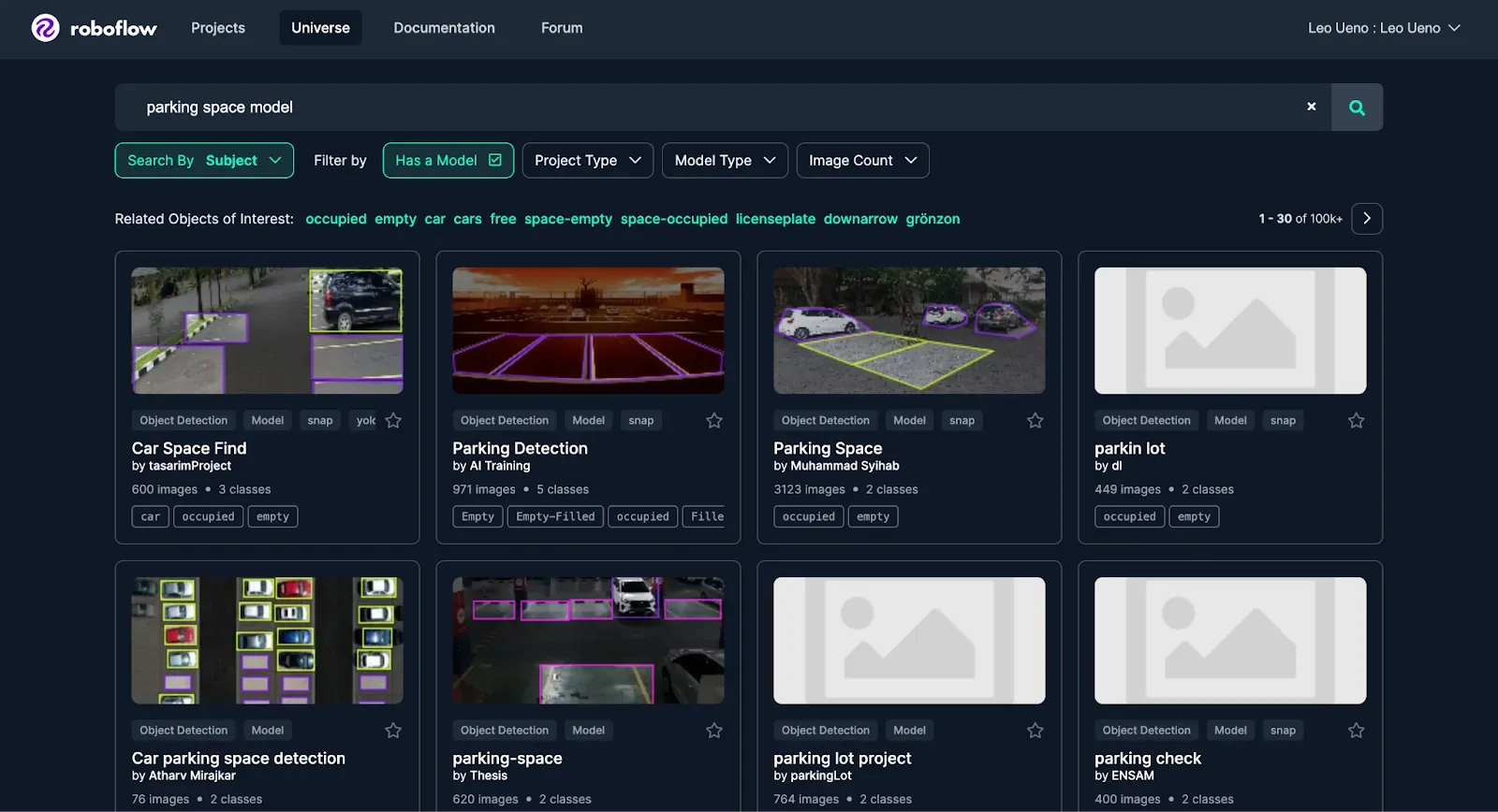
To get started, we will want to find a model that can be applied to our use case. We can search for a parking space model on Roboflow Universe to find a suitable model to detect occupied and empty parking spaces.
Make sure to test the model using a sample frame of our video to see if it would be suitable for our use case.
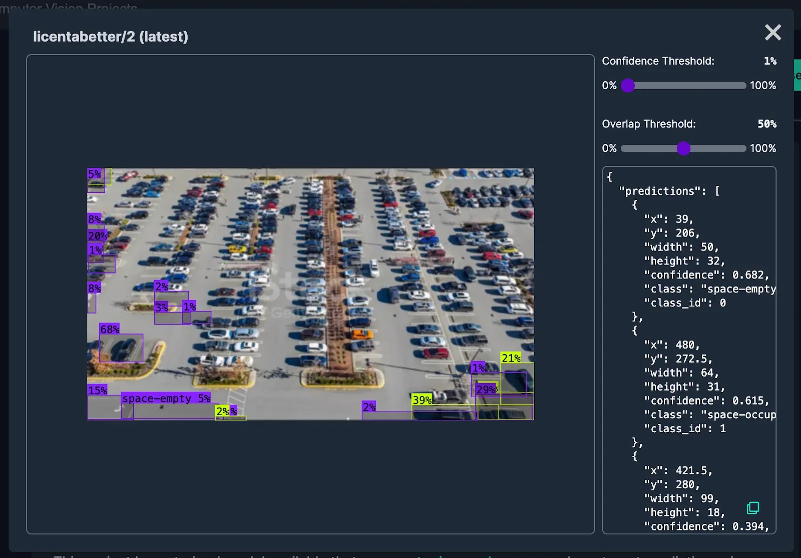
Unfortunately, this model and others that came up did not perform well for the footage we were planning to use. But, we can easily create a model to fit our use case.
Step 2: Creating and Training a Model
The first step in creating a computer vision model is to collect data. In our case, we have an example video that we can use. While other use cases may call for other model types, we have multiple objects we want to detect and we don’t need their exact shape, so we will use an object detection model.
Since our use case involves a very large number of small (relative to the entire image) objects, we will use a technique called Slicing Aided Hyper Inference (SAHI). SAHI allows us to predict in batches of smaller sections of the original image.
Collecting Images
First, we will use Supervision, an open-source computer vision utility, to extract the individual frames from the video, turning the videos into a set of images.
import supervision as sv
from PIL import Image


frames_generator = sv.get_video_frames_generator(VIDEO_PATH)


for i, frame in enumerate(frames_generator):
 img = Image.fromarray(frame)
 img.save(f"{FRAMES_DIR}/{i}.jpg")
When training a model, it’s important to train with data that is similar to what it will see when deployed. This will help boost performance.
Using SAHI means that our model will be seeing smaller sections of our example video, so we will randomly sample portions of our images to use for our training images. If you are not using SAHI, you can skip this step and upload the full frames.
# The full code for this script is available in the Colab notebook
source_folder = '/content/frames'
target_folder = '/content/augmented'
augment_images(source_folder, target_folder)
Once we have our training data, we can upload our images to Roboflow for annotation and training.
Automatic Labeling
Although we have the option to manually annotate our images, we will use automated image labeling in order to speed up the annotation process. Once we have our images uploaded, we can select the Auto Label Images option in the Assign page of our project.
Then, we will select images to test with and enter a prompt.
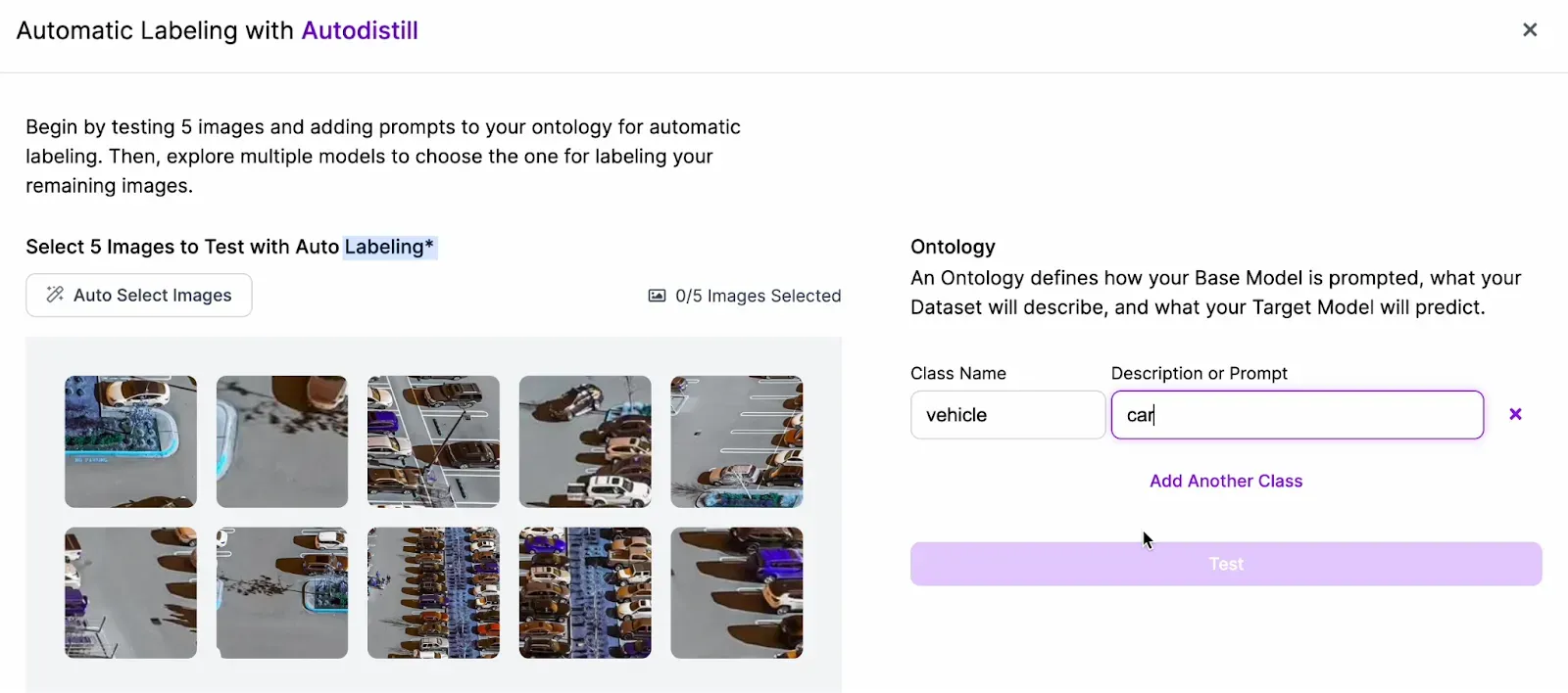
Looking through the model options with various confidence thresholds, we will pick the Grounding DINO model for labeling our dataset by copying the generated code for the respective model and running it in a Colab notebook or on your own device if you prefer.
Now that we have our dataset labeled, we can double-check for accuracy and correct any mistakes. Then, generate a version and start training the model.
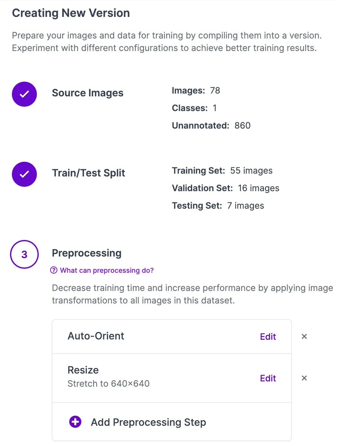
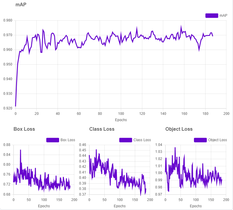
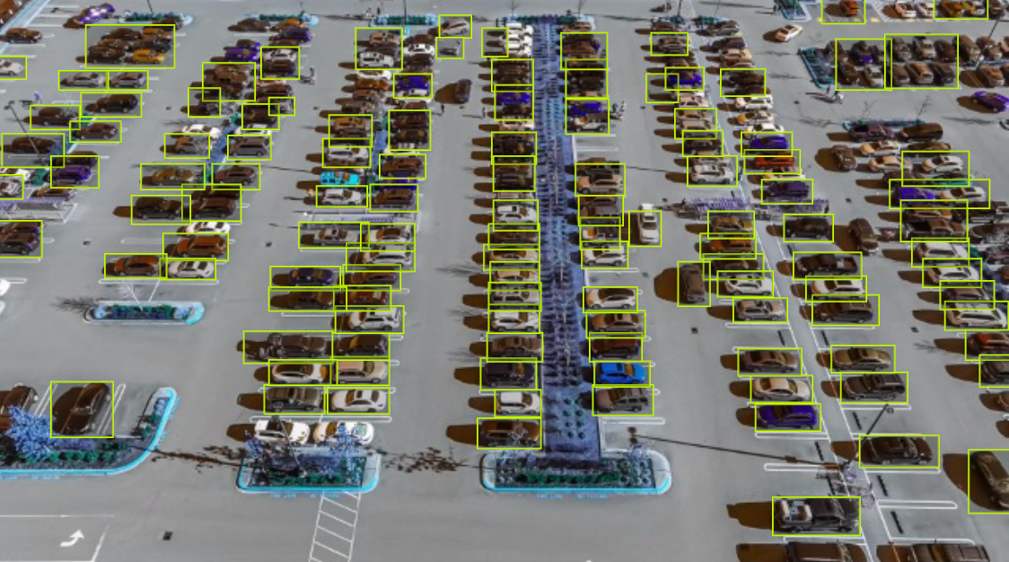
Our model finished with 96.9% mean average precision (mAP). By looking at a example prediction on one of our sample frames, we can see that it performs much better than the models we initially found, but it will work better once we use it with SAHI.
Step 3: Analyze Occupancy
Once our model has trained, or if there is a model that already works well to suit your use case, we can move on to analyzing the data.
To run a model on a video, we can create a callback function that will run on each frame. We will use this function in later steps to process predictions from our model.
from roboflow import Roboflow
import supervision as sv
import numpy as np
import cv2
rf = Roboflow(api_key="ROBOFLOW_API_KEY_HERE")
project = rf.workspace().project("parking-lot-occupancy-detection-eoaek")
model = project.version("5").model
def callback(x: np.ndarray) -> sv.Detections:
result = model.predict(x, confidence=25, overlap=30).json()
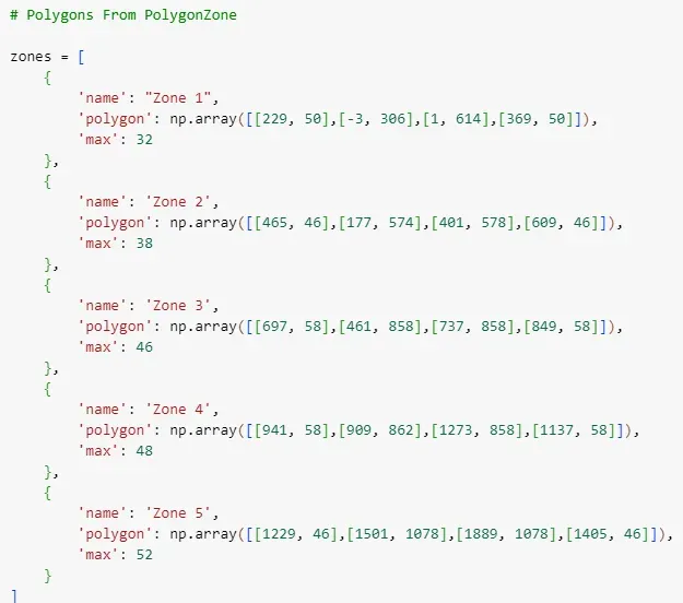
return sv.Detections.from_inference(result)Next, we will configure our detection zones. Supervision’s PolygonZone feature, which we will use to detect the vehicles in each zone of the parking lot, requires a set of points in order to identify where the zone is located, which can be generated using this online utility.
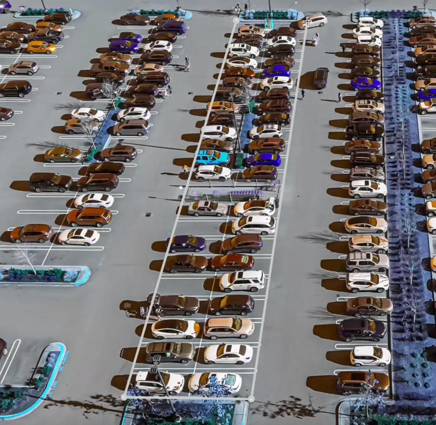
Once we upload a example frame from our video and get the coordinates for our zone, in order to make it as easy as possible to calculate our metrics later, we will create an array with the name of the zone, the coordinates of the polygon zone and a number for the parking spaces in the zone, so that we can calculate percentage occupancy later. We can now move on to the next step of setting up Supervision.
For our use case, we will use the following features of Supervision:
- ByteTrack: To track the location of our vehicles, so we can assess how long they are parked
- InferenceSlicer: A helper utility to run SAHI on our model
- TriangleAnnotator: To help visualize the locations of the vehicles
- HeatMapAnnotator: To generate heatmaps so we can identify our busiest areas
- PolygonZone, PolygonZoneAnnotator: To help count and identify vehicles in our respective zones and the annotator to help visualize those zones.
Now that we have everything we need to start running our detections, let’s try on a single image to see how it works.
image = cv2.imread("./frames/5.jpg")
image_wh = (image.shape[1],image.shape[0])
setup_zones(image_wh)

annotated_image, heatmap = process_frame(image)

sv.plot_image(annotated_image)
sv.plot_image(heatmap)
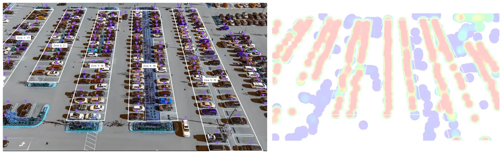
Checking the annotations marked on the image, it looks like everything is being detected properly. Next, we will process the entire video.
VIDEO_PATH = "/content/parkinglot1080.mov"
MAIN_OUTPUT_PATH = "/content/parkinglot_annotated.mp4"
frames_generator = sv.get_video_frames_generator(source_path=VIDEO_PATH)
video_info = sv.VideoInfo.from_video_path(video_path=VIDEO_PATH)

setup_zones(video_info.resolution_wh)

with sv.VideoSink(target_path=MAIN_OUTPUT_PATH, video_info=video_info) as sink:
  heatmap = None
  for i, frame in enumerate(frames_generator):
    print(f"Processing frame {i}")

    # Infer
    annotated_frame, heatmap = process_frame(frame, heatmap)
    sv.plot_image(annotated_frame)

    # Save the latest heatmap
    Image.fromarray(heatmap).save(f"/content/heatmap/{i}.jpg")

    # Create Graphs
    graphs = generate_graphs(video_info.total_frames)
    graph = graphs["combined_percentage"].convert("RGB")
    graph.save(f"/content/graphs/{i}.jpg")

    # Send as frame to video
    sink.write_frame(frame=annotated_frame)
Once the video has been processed, we can move on to extracting different metrics out of our results. We will cover: detecting the occupancy per zone, what percent of the spaces are occupied, the zones and specific areas in each zone that are the busiest and calculating how long people are parked in a space. See our guide to saving predictions to a Google Sheet if that's your preferred method for analysis.
Occupancy Per Zone
During our earlier setup process, we configured the number of detections in each zone to be recorded in a history array of each zone object. We can reference that number, as well as the max property in the zone to compare how occupied a single zone is.
import statistics
for zone in zones:
    occupancy_percent_history = [(count/zone['max'])*100 for count in zone['history']]
    average_occupancy = round(statistics.mean(occupancy_percent_history))
    median_occupancy = round(statistics.median(occupancy_percent_history))
    highest_occupancy = round(max(occupancy_percent_history))
    lowest_occupancy = round(min(occupancy_percent_history))
    print(f"{zone['name']} had an average occupancy of {average_occupancy}% with a median occupancy of {median_occupancy}%.")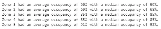
Additionally, during the video processing, these graphs were saved to the content/graphs folder. You can use the code in the Colab notebook to generate a video from the graphs in the folder, creating a video graphic demonstrating the occupancy percentage over time.
Total Occupancy
We can also evaluate the data to show us the total occupancy of the entire lot over the entire period.
lot_history = []
for zone in zones:
for idx, entry in enumerate(zone['history']):
if(idx >= len(lot_history) or len(lot_history)==0): lot_history.append([])
lot_history[idx].append(zone['history'][idx]/zone['max'])
lot_occupancy_history = [sum(entry)/len(entry)*100 for entry in lot_history]
average_occupancy = round(statistics.mean(lot_occupancy_history))
median_occupancy = round(statistics.median(lot_occupancy_history))
# ... other stats in Colab
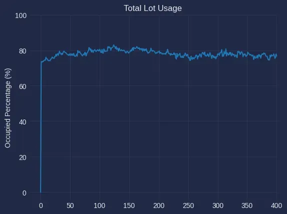
print(f"The entire lot had an average occupancy of {average_occupancy}% with a median occupancy of {median_occupancy}%.")By running this code, we can see the average and median occupancy, which both hovered around 78%.

We can get a good idea of the occupancy as a percentage, but it would also be useful to have access to the total lot occupancy over the entire period, output as a list for further analysis, or as a graph for visualization by accessing the lot_occupancy_history list we just created to calculate the average occupancy.
print(lot_occupancy_history)

# [
#    ...
#    73.34063105087132,
#    ...
# ]
By putting this list into a graph, we can see that occupancy remains fairly steady throughout the video recording period. While we have a steady amount through this short clip, using this process with video footage from the entire day or week, could provide insight into congestion trends.
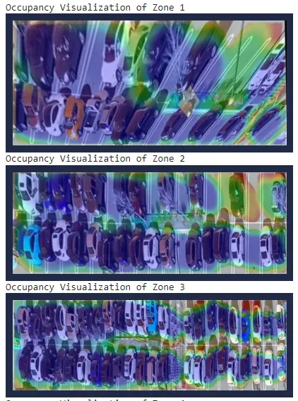
Busy Areas
With the images from the Supervision heatmap and the graphs that depict occupancy rates by zone, we can see where the busy areas are and where space may be underutilized.
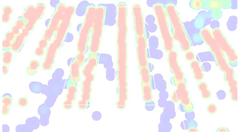
But, we can go a little bit further to create more visualizations. Since we already have the points for our zones, we can use them to rearrange our image to get a clearer view of which spaces in each of our zones are being underutilized.
Conclusion
These metrics and graphics that we created today show just a small portion of the possibilities that exist for data analytics with computer vision. For example, with a longer video, it would be possible to plot out when the busiest times of the day or week are, and perhaps share those insights in order to reduce congestion. We encourage you to use this guide as a starting point to build your own occupancy analytics system.
If you need assistance building your own occupation analytics system, contact the Roboflow sales team. Our sales team are experts in developing custom computer vision solutions for use cases across industry, from logistics to manufacturing to analytics.
Cite this Post
Use the following entry to cite this post in your research:
Leo Ueno. (Jan 31, 2024). Occupancy Analytics with Computer Vision. Roboflow Blog: https://blog.roboflow.com/occupancy-analytics/