
The Challenge of Ball Detection and Tracking
Ball tracking is an important feature for AI systems to analyze sports like soccer or basketball, enabling insights into player movements, strategies, and game dynamics. However, accurately detecting and tracking a ball in real-time is challenging.
Several factors contribute to the difficulty of ball tracking:
- Small size: The ball often occupies only a small portion of the image or video frame. It is especially difficult for the detector when the ball is far from the camera as it will be only a few pixels wide.
- High velocity: Balls in sports like soccer and tennis move very fast. This makes it difficult for trackers to accurately predict trajectories and handle sudden changes in direction. Additionally, the ball can be blurry in frames when it moves particularly fast, making it harder for the object detector to accurately locate.
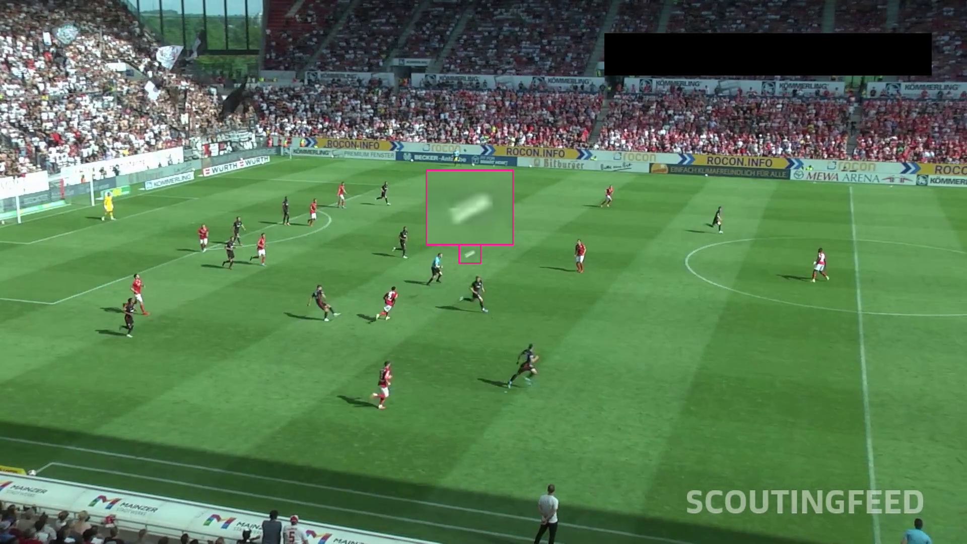
- Complex backgrounds: Live sports events often have cluttered backgrounds, particularly in soccer, when the ball is high in the air amidst spectators.
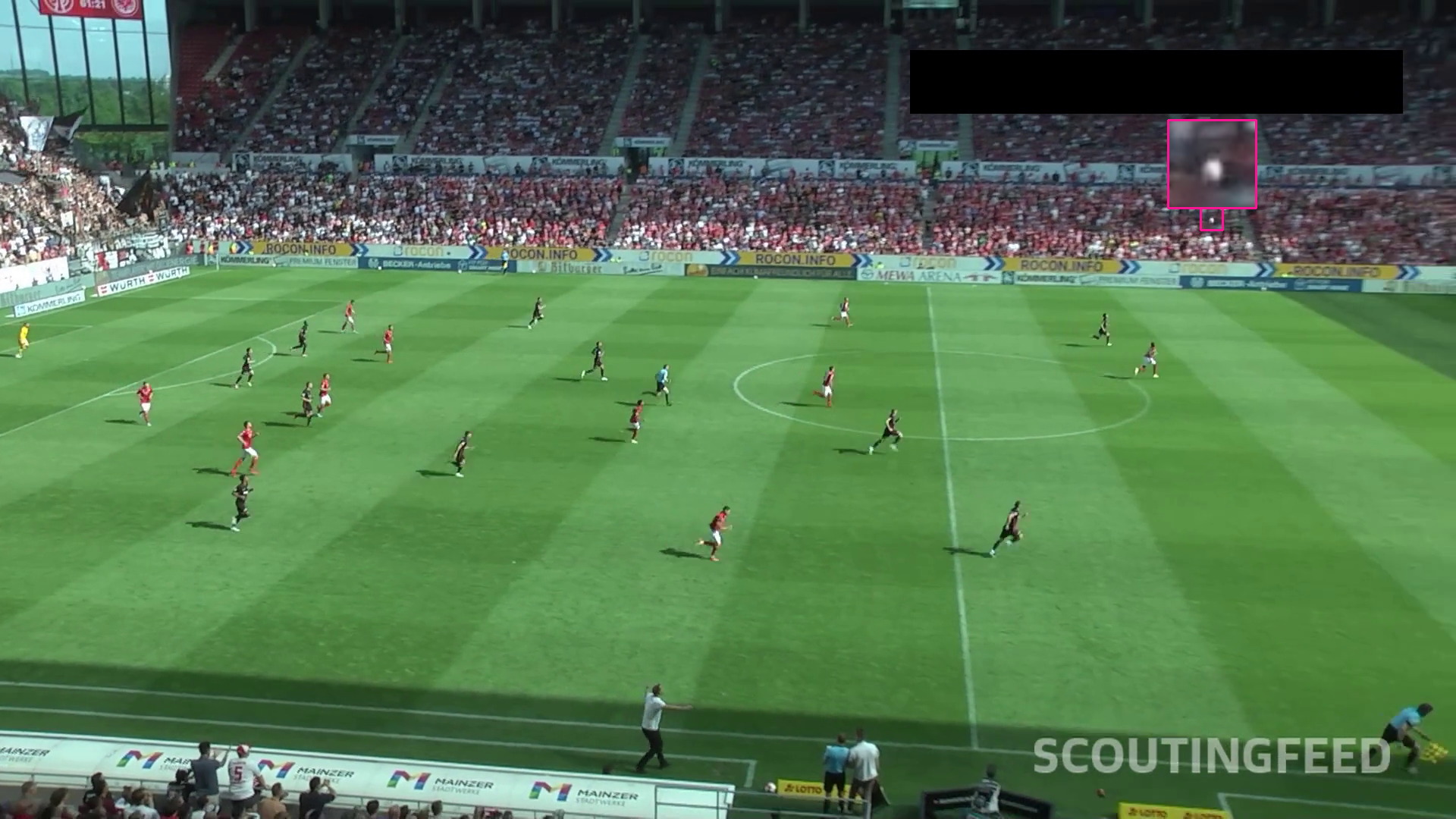
- Similar-looking objects: Many objects on the field or court resemble the ball, like player heads or other equipment. Sometimes there are even multiple balls on the same field.
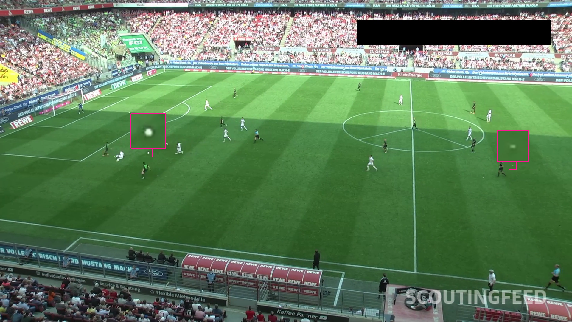
- Varying lighting conditions: Stadium lighting can be inconsistent, with shadows and glare affecting ball visibility. This requires robust algorithms that can adapt to different lighting scenarios.
In this tutorial, we'll tackle these challenges and teach the computer to track the ball effectively.
Ball Detection Model Training
The first step in building a soccer ball tracking application is to train a model. To do this, we need a suitable dataset. The original data for this project comes from the DFL - Bundesliga Data Shootout Kaggle competition. Videos were split into frames at a frequency of 3 per second and uploaded to Roboflow for annotation. The dataset must include images depicting the challenging cases described above.
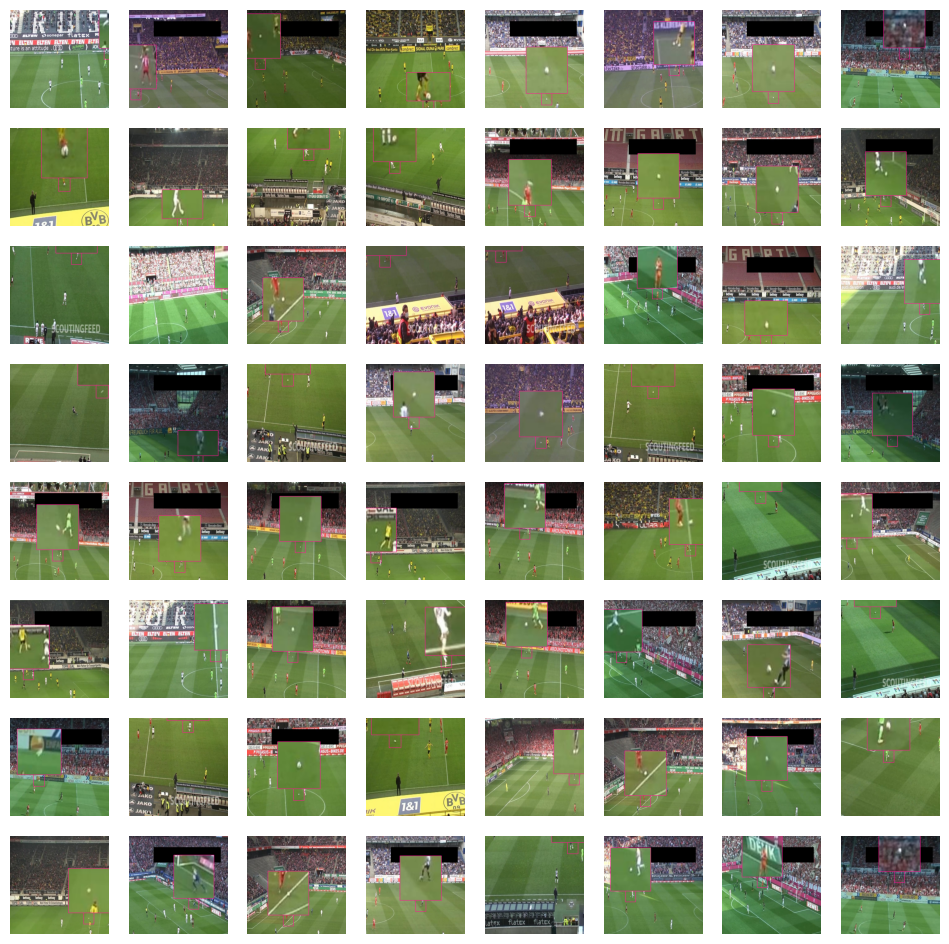
Next, we applied two preprocessing steps: we divided each video frame into 2x2 tiles and stretched each of those tiles to 640x640 resolution. This was done to increase the relative size of the ball within each tile and to standardize the input size for the model.
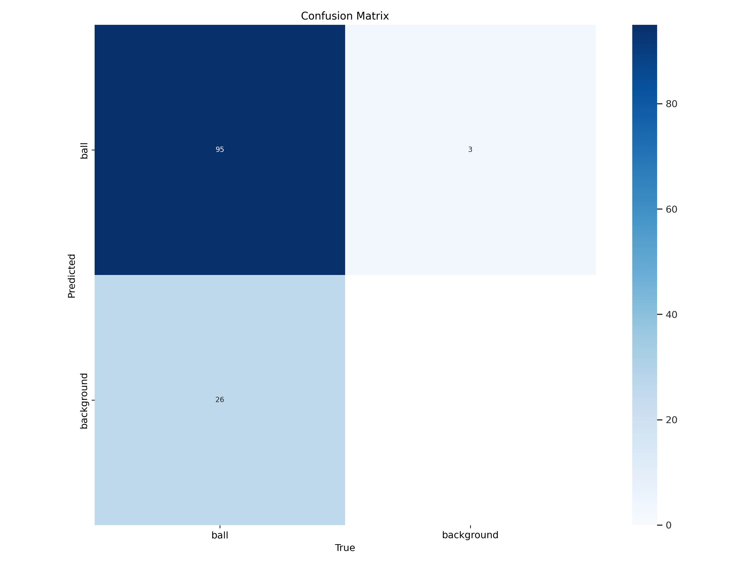
Based on this prepared dataset, we trained a YOLOv8x model for 50 epochs and, after completing the training, uploaded it to Roboflow. We achieved a mAP@0.50 of 0.925 and a mAP@0.5-95 of 0.57. A confusion matrix, which summarizes the model's prediction results, shows that the model still often makes mistakes, especially false negatives.
Detecting Small Objects in Sports
To load our trained model, you'll need the Inference and Supervision packages. Install them using:
pip install inference supervisionThen, you can load the custom football-ball-detection-rejhg/4 model and run it on a single image or video frame:
import supervision as sv
from inference import get_model

model = get_model(
    model_id="football-ball-detection-rejhg/4",
    api_key=<ROBOFLOW_API_KEY>
)

result = model.infer(frame, confidence=0.3)[0]
detections = sv.Detections.from_inference(result)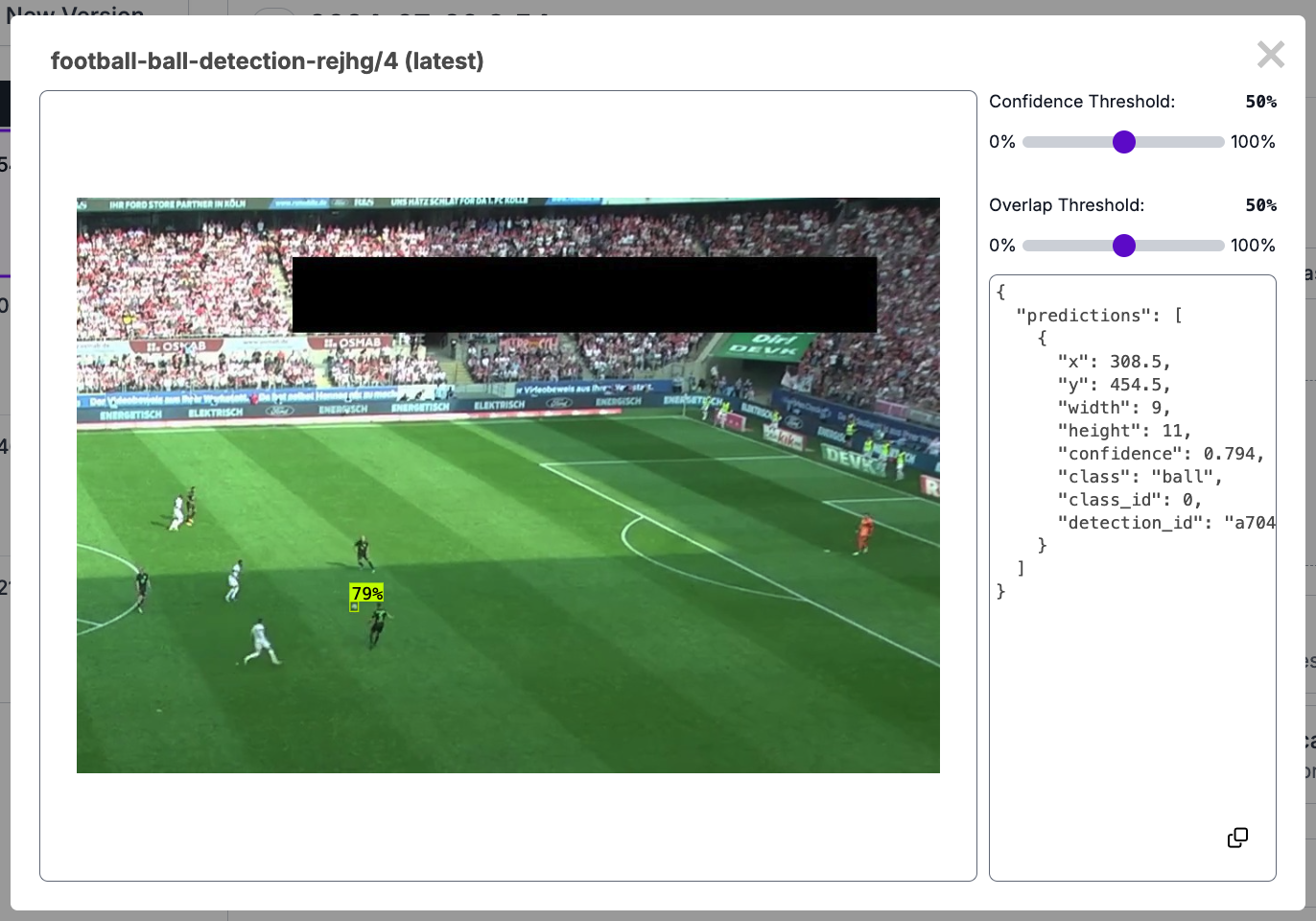
Before performing inference, computer vision models typically preprocess the image. One of the preprocessing steps is resizing the image to the input resolution imposed by the model's architecture.
In our case, we trained the model on 640x640. This is particularly problematic in the case of detecting small objects like a ball, which after resizing the frame to the expected resolution may shrink to barely a few pixels. As a result, they are too small to be detected effectively.
To address this, we use InferenceSlicer, which divides the image into smaller patches and performs inference on each patch separately. This effectively makes the ball proportionally larger within each patch, improving detection accuracy. However, it comes at the cost of reduced speed, as the model needs to run multiple times per frame.
import supervision as sv

def callback(patch: np.ndarray) -> sv.Detections:
    result = model.infer(patch, confidence=0.3)[0]
    return sv.Detections.from_inference(result)

h, w, _ = frame.shape

slicer = sv.InferenceSlicer(
    callback = callback,
    overlap_filter = sv.OverlapFilter.NON_MAX_SUPPRESSION,
    slice_wh = (w // 2 + 100, h // 2 + 100),
    overlap_ratio_wh = None,
    overlap_wh = (100, 100),
    iou_threshold = 0.1
)

detections = slicer(frame)To ensure smooth tracking between tiles, they overlap. If the ball is in the overlap and detected on two tiles simultaneously, InferenceSlicer will apply non-max suppression to eliminate redundant detections. Non-max suppression is an algorithm commonly used in object detection tasks to select the best bounding box out of a set of overlapping boxes. This helps reduce false positives and improve the overall accuracy of the detection.
Handling Anomalies for Ball Tracking
The soccer ball often gets misidentified due to its round shape and lack of distinct features.
To filter out these errors and locate the ball, the update method in BallTracker takes detection results, converts bounding boxes to center points, and stores them in a buffer. It then calculates the average ball position (centroid) and selects the ball closest to it, assuming there's only one ball on the field and its movement is physically realistic.
from collections import deque

class BallTracker:
    def __init__(self, buffer_size: int = 10):
        self.buffer = deque(maxlen=buffer_size)

    def update(self, detections: sv.Detections) -> sv.Detections:
        xy = detections.get_anchors_coordinates(sv.Position.CENTER)
        self.buffer.append(xy)

        if len(detections) == 0:
            return detections

        centroid = np.mean(np.concatenate(self.buffer), axis=0)
        distances = np.linalg.norm(xy - centroid, axis=1)
        index = np.argmin(distances)
        return detections[[index]]
This is just the basic logic, but it can potentially be extended to include a maximum allowable distance of the ball from the averaged position or predict the ball's position for video frames when no ball is detected. Another potential update could involve using a weighted average for the centroid calculation, giving more importance to recent detections.
Visualize Ball Tracking Results
To visualize our ball tracking results, we combine the previous steps: loading the model, slicing the frame, running inference, filtering with the tracker, and annotating the frame. On top of that, we add TriangleAnnotator - one of the annotators available in supervision, which will allow us to obtain the ball tracking view known from computer games.
import supervision as sv
from inference import get_model

model = get_model(
    model_id="football-ball-detection-rejhg/4",
    api_key=<ROBOFLOW_API_KEY>
)

video_info = sv.VideoInfo.from_video_path(<SOURCE_PATH>)
frame_generator = sv.get_video_frames_generator(<SOURCE_PATH>)
w, h = video_info.width, video_info.height

def callback(patch: np.ndarray) -> sv.Detections:
    result = model.infer(frame, confidence=0.3)[0]
    return sv.Detections.from_inference(result)

slicer = sv.InferenceSlicer(
    callback = callback,
    overlap_filter = sv.OverlapFilter.NON_MAX_SUPPRESSION,
    slice_wh = (w // 2 + 100, h // 2 + 100),
    overlap_ratio_wh = None,
    overlap_wh = (100, 100),
    iou_threshold = 0.1
)

annotator = sv.TriangleAnnotator(
    color=sv.Color.from_hex('#FF1493'),
    height=20,
    base=25
)

tracker = BallTracker()

with sv.VideoSink(<TARGET_PATH>, video_info=video_info) as sink:
    for frame in frame_generator:
        detections = slicer(frame)
        detections = tracker.update(detections)
        frame = annotator.annotate(scene=frame, detections=detections)
sink.write_frame(frame)The TriangleAnnotator provides a basic visualization, but we can create more customized annotators for a richer representation of ball movement. The BallAnnotator class is a good example. The implementation initializes a color palette from Matplotlib's "jet" colormap with a specified buffer size. It maintains a buffer to store recent ball positions.
The annotate method takes a frame and detections, updates the buffer with the current position, and draws circles for each position in the buffer, using interpolated radius and corresponding colors from the palette.
class BallAnnotator:
    def __init__(
        self,
        radius: int,
        buffer_size: int = 5,
        thickness: int = 2
    ):
        self.color_palette = sv.ColorPalette.from_matplotlib('jet', buffer_size)
        self.buffer = deque(maxlen=buffer_size)
        self.radius = radius
        self.thickness = thickness

    def interpolate_radius(self, i: int, max_i: int) -> int:
        if max_i == 1:
            return self.radius
        return int(1 + i * (self.radius - 1) / (max_i - 1))

    def annotate(
        self,
        frame: np.ndarray,
        detections: sv.Detections
    ) -> np.ndarray:
        xy = detections.get_anchors_coordinates(
            sv.Position.BOTTOM_CENTER).astype(int)
        self.buffer.append(xy)

        for i, xy in enumerate(self.buffer):
            color = self.color_palette.by_idx(i)
            radius = self.interpolate_radius(i, len(self.buffer))

            for center in xy:
                frame = cv2.circle(
                    img=frame,
                    center=tuple(center),
                    radius=interpolated_radius,
                    color=color.as_bgr(),
                    thickness=self.thickness
                )
        return frame
Conclusions
In this tutorial, we explored the challenges of ball tracking in sports and demonstrated how to build a basic ball detection and tracking system using Python, inference, and supervision libraries.
We covered model loading, image slicing for improved detection, anomaly handling with a simple tracker, and visualization using both built-in and custom annotators. This system can be further enhanced with more sophisticated tracking algorithms, additional filtering techniques, and refined visualizations to cater to specific sports and use cases.
Ball tracking is just one of the components needed to create a soccer AI. Check out our sports repository to learn what else can be done by combining computer vision and sports.
Cite this Post
Use the following entry to cite this post in your research:
Piotr Skalski. (Aug 6, 2024). Ball Tracking in Sports with Computer Vision. Roboflow Blog: https://blog.roboflow.com/tracking-ball-sports-computer-vision/