
RF-DETR Keypoint is a real-time transformer model for keypoint detection. It extends the RF-DETR architecture, which is already state-of-the-art for object detection and instance segmentation. The model predicts bounding boxes and keypoint coordinates in a single forward pass, with no NMS and no heatmaps. Each keypoint comes with confidence scores and an uncertainty ellipse derived from a learned covariance matrix.
The default checkpoint is trained on COCO person pose with 17 keypoints. RF-DETR Keypoint is not limited to that skeleton: you can fine-tune on any keypoint layout attached to any object class. In this tutorial, we walk through that fine-tuning workflow step by step.
You can follow along interactively. All code blocks in this tutorial are ready to run in our companion notebook.
To demonstrate the fine-tuning process, we will train a custom court detector using basketball-court-detection-2. This dataset provides 33 landmarks mapped to specific locations on a basketball court. We will walk through the entire pipeline, from initializing the Preview checkpoint to evaluating the model on held-out test images and NBA broadcast footage.
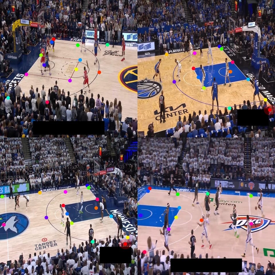
The fine-tuned RF-DETR Keypoint model running inference on unseen NBA broadcast footage, successfully tracking 33 court landmarks despite heavy occlusion.
Run RF-DETR Keypoint Preview on COCO
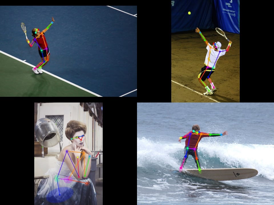
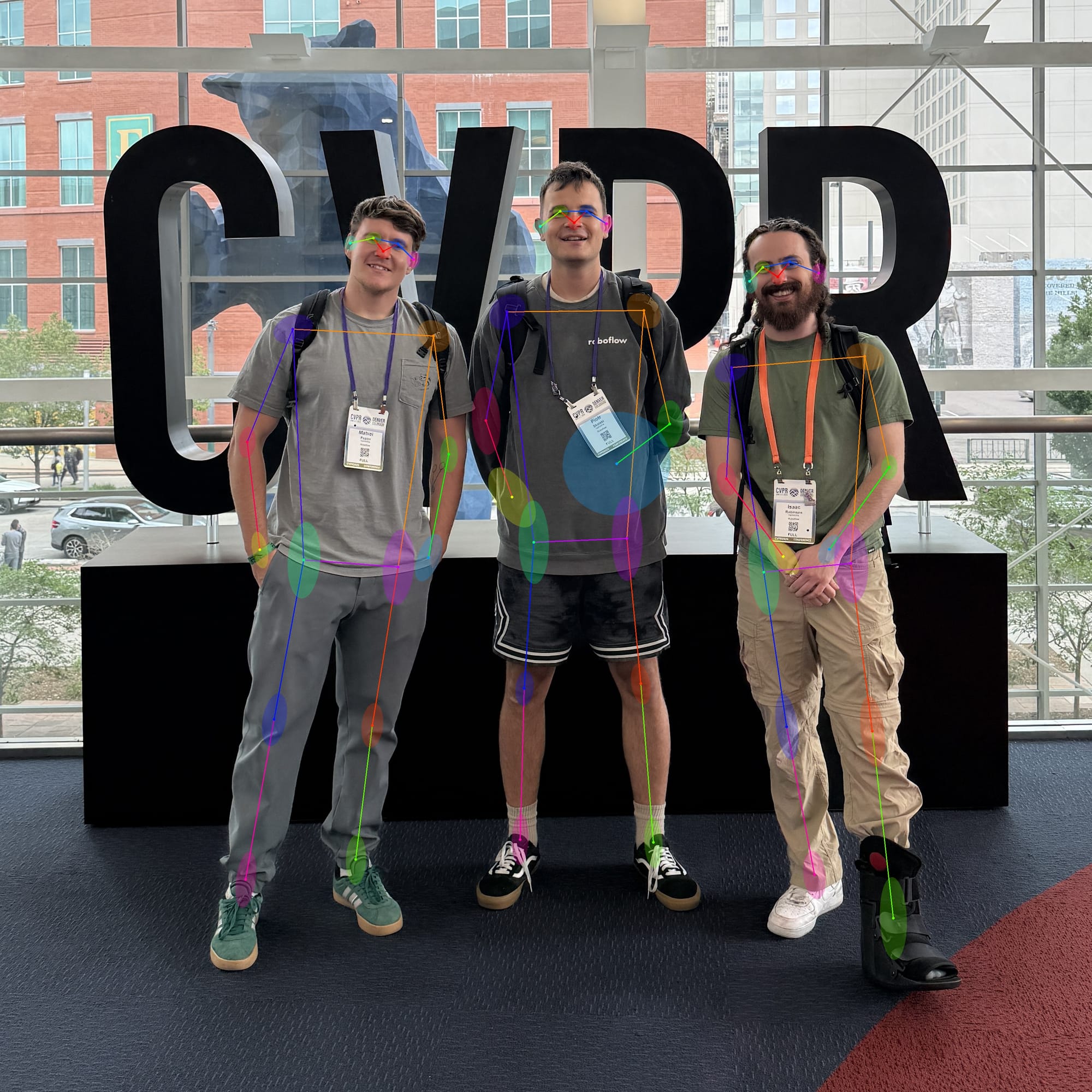
Run the COCO Preview checkpoint on a sample image before fine-tuning. You get instance boxes, 17 body keypoints, and per-joint confidence scores for each detection. The model also predicts a covariance matrix for each keypoint, which supervision renders as uncertainty ellipses. Use the code below to predict and visualize the result.
import cv2
import supervision as sv
from rfdetr import RFDETRKeypointPreview

IMAGE_PATH = "<PATH_TO_IMAGE>"

model = RFDETRKeypointPreview()
key_points = model.predict(IMAGE_PATH, threshold=0.5).with_nms()

image = cv2.imread(IMAGE_PATH)

edge_annotator = sv.EdgeAnnotator(color=sv.Color.ROBOFLOW, thickness=2)
ellipse_annotator = sv.VertexEllipseAnnotator(sigma=2.0, color=sv.Color.ROBOFLOW, max_axis=36.0)
vertex_annotator = sv.VertexAnnotator(radius=4, color=sv.Color.ROBOFLOW)

image = edge_annotator.annotate(scene=image, key_points=key_points)
image = ellipse_annotator.annotate(scene=image, key_points=key_points)
image = vertex_annotator.annotate(scene=image, key_points=key_points)

sv.plot_image(image)
Load the pre-trained model, run inference on a sample image, and visualize the resulting keypoints and uncertainty ellipses.
Build Your COCO Keypoint Dataset
When building a custom keypoint dataset in Roboflow Annotate, consistency is critical. For the basketball court, every one of the 33 points must be placed at its exact geometric location (like a specific lane corner or line intersection) across all frames. This ensures the model learns the true spatial structure regardless of the camera angle. See the keypoint detection guide for skeleton setup.
In Roboflow Annotate, use visible when the court feature appears in the image and occluded when it is hidden but geometrically known. Skip points that are off-screen entirely. COCO stores that as visibility per triplet: v=2 visible, v=1 occluded, v=0 not in the annotation.
Your training data must be exported in COCO Keypoint format so the code can read these visibility flags correctly. Every annotated object carries a sequence of x, y, and visibility values for each named keypoint in your skeleton. Generate a dataset version from Roboflow Annotate as COCO Keypoint JSON. Each split folder will then contain images plus _annotations.coco.json.
Fine-tuning initializes from the same Preview checkpoint you ran above. You replace the default 17-keypoint person head configuration with num_keypoints_per_class and class_names from your annotation JSON. For basketball, that means 33 court landmarks on the court class. From here, you have two options: train the model with no code using the Roboflow platform, or write a custom training loop using our open source Python package.
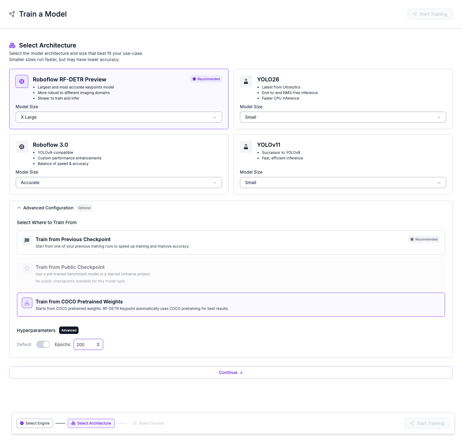
Train on Roboflow
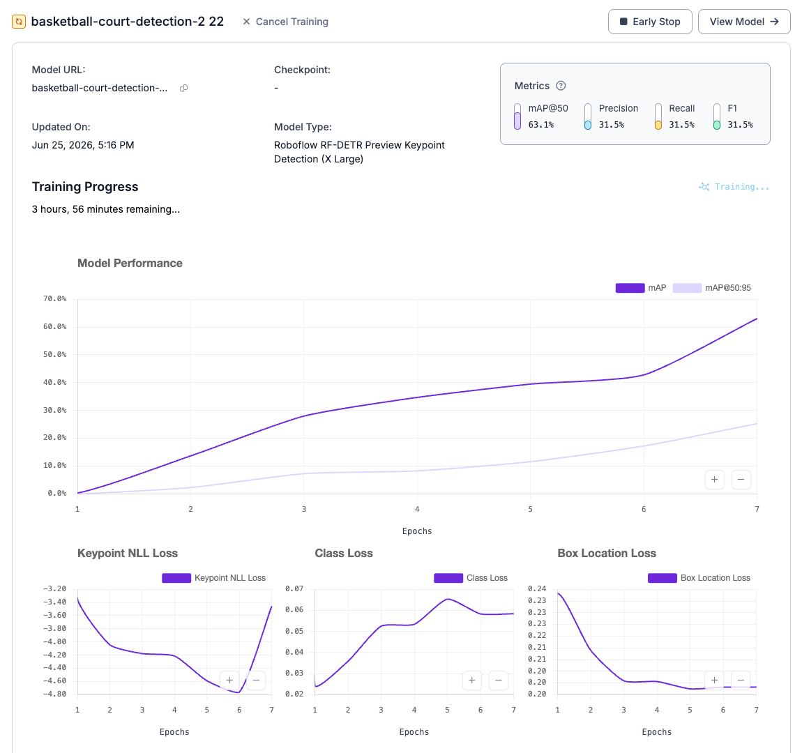
If you prefer a no-code approach, you can train RF-DETR Keypoint directly within the Roboflow platform. After labeling your dataset, navigate to the Train tab and select the Roboflow RF-DETR Preview architecture. The Preview release currently uses the X Large model size. You can choose to start from COCO pre-trained weights or a checkpoint you previously trained to speed up convergence.
Before training begins, configure your dataset preprocessing. Standardize your images by applying Auto-Orient and resizing them to 576x576 to match the model's native input resolution. Once you generate the dataset version, review the summary and click Start Training.
The platform handles the infrastructure and hyperparameter optimization automatically. As the model trains, you can monitor live progress charts tracking keypoint mAP, Precision, Recall, and various loss metrics. You can let the training run for the full duration or use the Early Stop feature if the metrics stabilize. Once training is complete, your model is immediately available for deployment via the Roboflow API.
Train with the Open Source Python Package
Install Dependencies
Run the pip command below in Colab or your local virtual environment. Use rfdetr>=1.8.1 with the train and visual extras and supervision>=0.29.1 for Keypoint Preview training and ellipse visualization. Add roboflow for Universe download.
pip install "rfdetr[train,visual]>=1.8.1" roboflow "supervision>=0.29.1"Download the Dataset
Pull the public basketball court dataset from Universe using the Roboflow SDK below. Choose the COCO export format. The SDK extracts three splits under DATASET_DIR, each with paired images and _annotations.coco.json.
from pathlib import Path
from roboflow import Roboflow

rf = Roboflow()
dataset = (
    rf.workspace("roboflow-jvuqo")
    .project("basketball-court-detection-2")
    .version(19)
    .download("coco", location="datasets/basketball_court")
)
DATASET_DIR = Path(dataset.location)
Use the Roboflow SDK to download the basketball court dataset in COCO Keypoint format and set the dataset directory path.
Configure API Key
The download cell above uses your Roboflow API key from the environment. In Colab, store it under Secrets as ROBOFLOW_API_KEY. Locally, export the same variable in your shell before re-running the download snippet.
Fine-Tune RF-DETR Keypoints on Your Dataset
Infer Your Keypoint Schema
Your annotation file defines how many keypoints each class has and what the classes are called. The helper below extracts that structure so you do not hard-code numbers that drift when the dataset changes. Keep NUM_CLASSES, NUM_KEYPOINTS_PER_CLASS, and KEYPOINT_OKS_SIGMAS for the inference section later.
from rfdetr.datasets._keypoint_schema import infer_coco_keypoint_schema

schema = infer_coco_keypoint_schema(DATASET_DIR / "train" / "_annotations.coco.json")
CLASS_NAMES = schema.class_names
NUM_KEYPOINTS_PER_CLASS = schema.num_keypoints_per_class
NUM_CLASSES = len(CLASS_NAMES)
KEYPOINT_OKS_SIGMAS = schema.keypoint_oks_sigmas
Extract the class names, keypoint counts, and Object Keypoint Similarity (OKS) sigmas directly from the COCO annotations to avoid hardcoding schema details.
Configure Training
A Colab T4 is sufficient for this tutorial. Set RESOLUTION = 576 to match the Preview input size. The hyperparameter block below sets BATCH_SIZE=2 and GRAD_ACCUM_STEPS=2 for that hardware profile. EPOCHS, BATCH_SIZE, and GRAD_ACCUM_STEPS control training length and effective batch size. A larger GPU can take a higher batch size without lowering resolution.
Gradient accumulation lets you train with large-batch stability on a small GPU. With BATCH_SIZE=2 and GRAD_ACCUM_STEPS=2, each optimizer step averages gradients over four images. Increase GRAD_ACCUM_STEPS if you want a larger effective batch without raising memory use.
OUTPUT_DIR = "output/keypoint_basketball_court_detection_demo"

RESOLUTION = 576
EPOCHS = 50
BATCH_SIZE = 2
GRAD_ACCUM_STEPS = 2
LR = 1e-4
Define the output directory and set the training hyperparameters, including resolution, epochs, batch size, and learning rate.
Fine-Tune the Model
The code block below initializes the model with your custom schema and starts the training loop. trainer.fit handles the optimization process, automatically saving the best weights to checkpoint_best_total.pth. All training and validation scalars are logged to metrics.csv in your output directory for later analysis.
Timelapse of model predictions (solid dots) converging toward ground truth labels (hollow rings) across 4 validation images during training.
from rfdetr import RFDETRKeypointPreview
from rfdetr.config import KeypointTrainConfig
from rfdetr.training import RFDETRDataModule, RFDETRModelModule, build_trainer

variant = RFDETRKeypointPreview(
    num_classes=NUM_CLASSES,
    num_keypoints_per_class=NUM_KEYPOINTS_PER_CLASS,
    resolution=RESOLUTION,
)
train_config = KeypointTrainConfig(
    dataset_file="roboflow",
    dataset_dir=str(DATASET_DIR),
    output_dir=OUTPUT_DIR,
    epochs=EPOCHS,
    batch_size=BATCH_SIZE,
    grad_accum_steps=GRAD_ACCUM_STEPS,
    lr=LR,
    lr_encoder=LR,
    class_names=CLASS_NAMES,
    keypoint_oks_sigmas=KEYPOINT_OKS_SIGMAS,
)
datamodule = RFDETRDataModule(variant.model_config, train_config)
model_module = RFDETRModelModule(variant.model_config, train_config)
trainer = build_trainer(train_config, variant.model_config)
trainer.fit(model_module, datamodule=datamodule)
Initialize the model and training configuration and start the fine-tuning process.
Evaluate Training Results
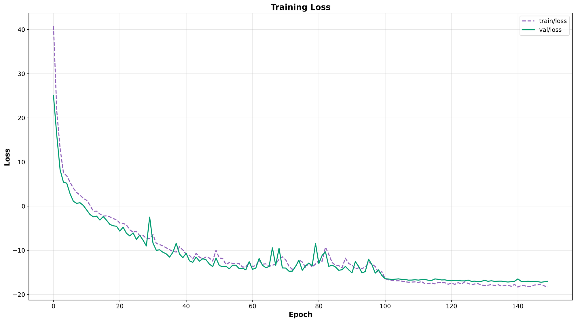
The plot helpers below visualize the data recorded in metrics.csv. The most important metric for checkpoint selection is val/keypoint_map_50_95. A widening gap where training loss drops but validation keypoint mAP stalls is a clear indicator of overfitting to the training set.
metrics.csv.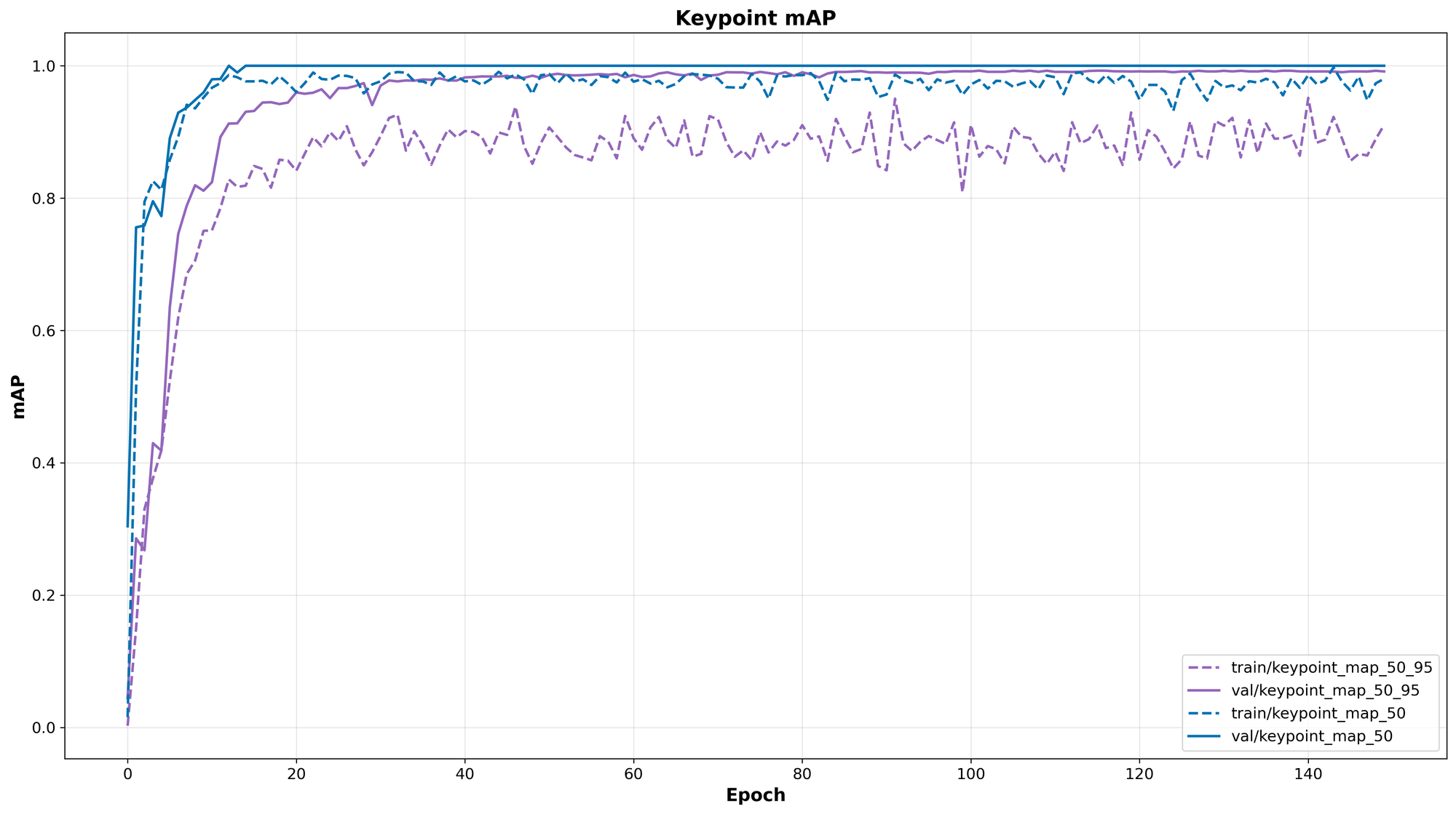
metrics.csv.from rfdetr.visualize.training import plot_loss_metrics, plot_map_metrics
plot_loss_metrics(f"{OUTPUT_DIR}/metrics.csv")
plot_map_metrics(f"{OUTPUT_DIR}/metrics.csv")Generate visualizations of the training loss and validation mAP curves from the logged CSV metrics.
Timelapse frames replay the same eval images through checkpoints saved during training. Predictions start far from labels and improve epoch over epoch. Ellipse size shrinks as the model gains confidence on each court feature. Colored dots are model output; hollow rings are ground truth in the clips below.
Epoch-by-epoch convergence on a single validation frame: uncertainty ellipses shrink as the model gains confidence in the court geometry.
Some eval frames show predictions where no ground-truth point was labeled. That happens when the broadcast crop cuts off part of the court, when a point was left off-screen during annotation, or when crowd occlusion made the feature hard to label. The model may still emit a low-confidence keypoint with a large uncertainty ellipse. Compare ellipse size and confidence, not label overlap alone, on those frames.
Run Inference with Your Fine-Tuned Model
Load Your Checkpoint
Load your best checkpoint with RFDETRKeypointPreview.from_checkpoint. Pass the same num_classes and num_keypoints_per_class you used during training so the head shapes match the saved weights. The path below points to checkpoint_best_total.pth in your output directory.
loaded_model = RFDETRKeypointPreview.from_checkpoint(
    f"{OUTPUT_DIR}/checkpoint_best_total.pth",
    num_classes=NUM_CLASSES,
    num_keypoints_per_class=NUM_KEYPOINTS_PER_CLASS,
)
Load the best saved checkpoint using the exact same class and keypoint schema configuration used during training.
Run Inference on a Test Image
One forward pass returns court boxes and 33 keypoints with covariance. Apply bbox and keypoint thresholds before calling the supervision annotators. Filter weak joints using keypoint confidence before drawing. The snippet below loads a test frame and plots the result.
import cv2
import supervision as sv

IMAGE_PATH = "<PATH_TO_IMAGE>"

key_points = loaded_model.predict(IMAGE_PATH, threshold=0.5).with_nms()

image = cv2.imread(IMAGE_PATH)

ellipse_annotator = sv.VertexEllipseAnnotator(sigma=1.0, max_axis=36.0)
vertex_annotator = sv.VertexAnnotator(radius=3, color_lookup=sv.ColorLookup.KEYPOINT)

image = ellipse_annotator.annotate(scene=image, key_points=key_points)
image = vertex_annotator.annotate(scene=image, key_points=key_points)

sv.plot_image(image)
Run a forward pass on a test image, filter the keypoints by confidence, and render the predictions using supervision annotators.
The fine-tuned RF-DETR Keypoint model running inference on unseen NBA broadcast footage, successfully tracking 33 court landmarks despite heavy occlusion.
What You Can Build Next
With a reliable court keypoint model, you can map broadcast video directly to a 2D tactical board. This homography transformation turns raw video into structured spatial data. Combine it with tracking models to render player radars and visualize tactical formations.
Conclusion
This tutorial walked from pre-trained keypoint detection to a custom basketball court model. You fine-tuned RF-DETR Keypoint on a Roboflow dataset, reviewed training metrics, and ran inference with your saved checkpoint. Repeat the same steps with your own skeleton and dataset.
Fork the notebook, point the download cell at your Roboflow project, and start training on your own data. You can run this fine-tuning pipeline using our open source repository or train directly within the Roboflow platform. As you expand your computer vision projects, remember that RF-DETR is also the state-of-the-art model for object detection and instance segmentation.
Cite this Post
Use the following entry to cite this post in your research:
Piotr Skalski. (Jun 26, 2026). How to Fine-Tune RF-DETR Keypoints on Custom Data. Roboflow Blog: https://blog.roboflow.com/train-rf-detr-keypoint/