What Is Promptable Concept Segmentation (PCS)?

Segmentation models in computer vision are designed to understand the structure of a scene by assigning pixel-level labels to objects. Traditional approaches such as semantic, instance, and panoptic segmentation provide detailed maps of where things are and what they belong to. These methods are widely used in applications such as autonomous navigation and medical imaging.

However, existing segmentation models work with a predefined set of object categories (labels). If an object is not part of that list, the model cannot segment it. These models also run one full inference pass per query, which limits flexibility. As vision systems begin to integrate language understanding, a more flexible approach has been introduced, known as Promptable Concept Segmentation (PCS).

PCS avoids the restrictions of a fixed vocabulary and allows the model to segment objects described directly by a text prompt or example images. So, instead of limiting the model to predefined labels, PCS accepts prompts such as noun phrases (“red apple”) or example images.

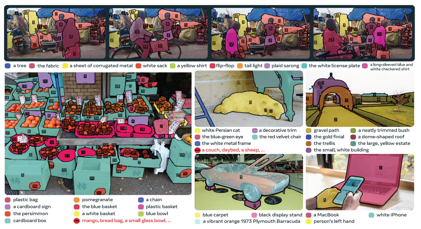
The model then returns segmentation masks for all instances of the described concept in an image or video. This makes segmentation more flexible, scalable, and aligned with how humans naturally describe visual concepts. The following image illustrates the concept of PCS.

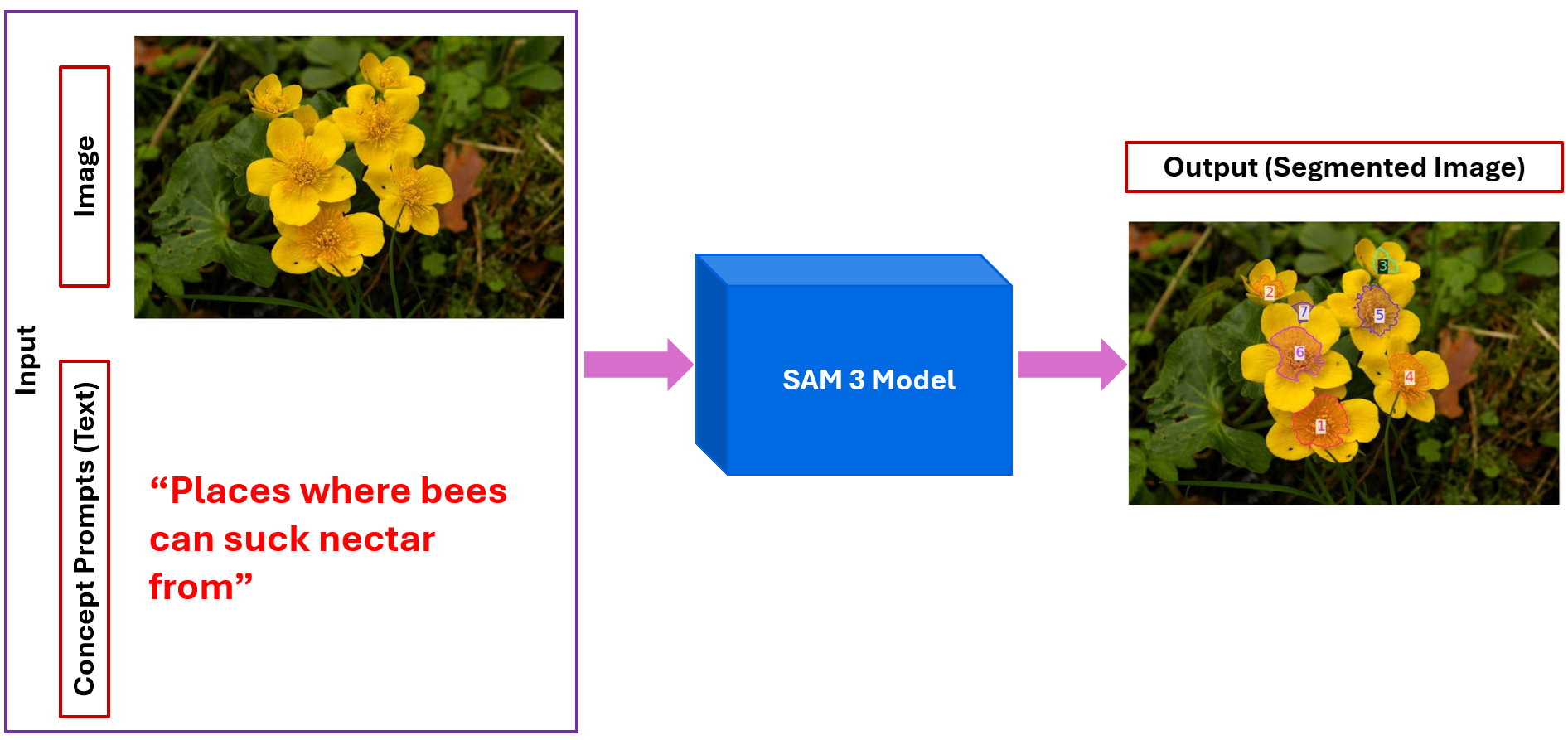
The image shows how SAM 3 uses a natural-language prompt to segment concepts in an image. The user provides the text “Places where bees can suck nectar from,” and SAM 3 identifies and segments all flower centers that match this description. The output highlights each instance separately, demonstrating prompt-controlled, open-vocabulary segmentation. This article explores:

• What PCS is
• Why it matters
• How PCS compares to semantic, instance, and panoptic segmentation
• The architecture of SAM 3, the third generation of the Segment Anything Model.
• The data and training system behind SAM 3.

At the end of this article you will have clear understanding about PCS and how PCS extends the capabilities of segmentation models.

What Is Promptable Concept Segmentation?

Promptable Concept Segmentation (PCS) generalizes interactive segmentation by allowing users to segment every object matching a concept instead of a single instance. The SAM 3 paper defines the PCS task as follows:

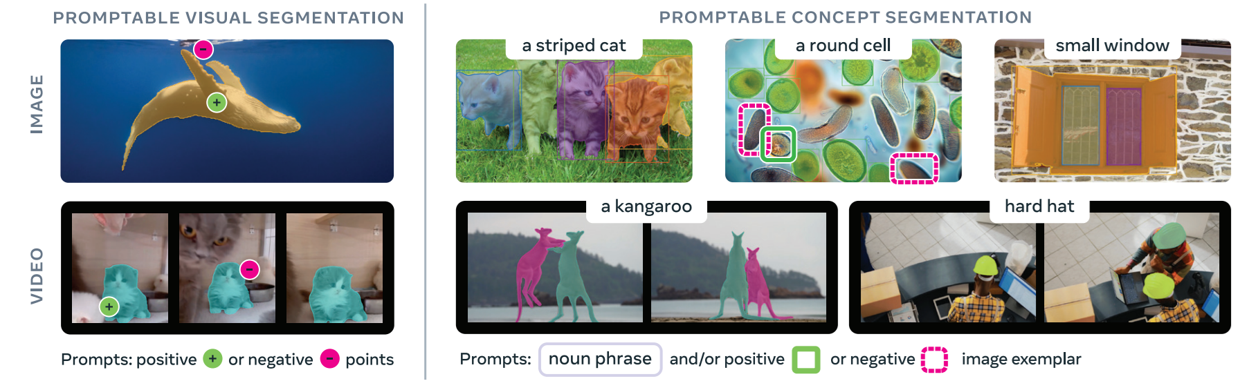
“Given an image or short video (≤30 secs), detect, segment, and track all instances of a visual concept specified by a short text phrase, image exemplars, or a combination of both.”

Here, concepts are restricted to simple noun phrases (NPs) consisting of a noun and optional modifiers. Text prompts are global across frames, while image exemplars can be provided on individual frames and can be positive or negative bounding boxes.

SAM 3 formalizes this by taking text and/or image exemplars as input and predicting instance and semantic masks for every object matching the concept while preserving object identities across video frames. In other words, PCS returns a set of masks (and optionally bounding boxes) for all objects that satisfy the user’s prompt.

Unlike traditional segmentation, PCS is prompt‑based and open‑vocabulary. Users provide a query in the form of a noun phrase or exemplar images, and the model segments all corresponding objects in the input. This is powerful for tasks where pre‑defined class lists fall short for example, segmenting “striped cat”, “yellow school bus” or “blue recycling bin” in an image or video. The SAM 3 paper highlights that PCS can be used to recognize atomic visual concepts like “red apple” or “striped cat”, enabling fine‑grained segmentation beyond standard categories.

Why Is Promptable Concept Segmentation So Impactful?

Open‑vocabulary segmentation unlocks new applications. Annotators can quickly label datasets by prompting for rare objects or specific attributes, robotic systems can interact with objects described by natural language, and creative tools can isolate elements defined by arbitrary descriptions. PCS also bridges vision and language: the prompt is expressed as text and/or images, and the model must align these modalities to produce accurate segmentation masks.

How PCS Is Different from Classic Segmentation Models

First we will cover semantic, instance, and panoptic segmentation, and then we will compare them with PCS, highlighting key differences.

Semantic Segmentation

Assigns every pixel a class label, but does not differentiate between multiple objects (instances) of the same class.

Key idea: It provides class-level labeling. All objects of the same class are treated as a single entity.

Example:

Try the following code.

sem_weights = FCN_ResNet50_Weights.COCO_WITH_VOC_LABELS_V1
sem_model = fcn_resnet50(weights=sem_weights).to(device).eval()
sem_classes = sem_weights.meta["categories"]

sem_transform = transforms.Compose([
    transforms.ToTensor(),
    transforms.Normalize(mean=[0.485, 0.456, 0.406],
                         std=[0.229, 0.224, 0.225])
])

sem_input = sem_transform(img_pil).unsqueeze(0).to(device)

with torch.no_grad():
    sem_logits = sem_model(sem_input)["out"]

sem_pred = sem_logits.argmax(1)[0].cpu().numpy().astype(np.int32)
sem_mask_color = colorize_id_mask(sem_pred, seed=1)

print("\n=== SEMANTIC SEGMENTATION DETECTED CLASSES ===")
for cid in np.unique(sem_pred):
    print(f"ID {cid:2d} → {sem_classes[cid]}")

plt.figure(figsize=(8, 8))
plt.imshow(sem_mask_color)
plt.axis("off")
plt.show()

The above code loads a pretrained FCN-ResNet50 model from torchvision.models.segmentation using FCN_ResNet50_Weights.COCO_WITH_VOC_LABELS_V1, which gives you both the network and the list of VOC-style class names (person, car, dog, etc.). The input image is first converted to a PyTorch tensor and normalized with ImageNet-style mean and std using torchvision.transforms.

This preprocessed tensor is passed through the FCN model in evaluation mode, producing a 4D output tensor with class scores for every pixel. The code then takes the argmax across the class dimension to get a 2D integer mask, where each pixel holds the ID of the most likely class. That ID mask is fed into colorize_id_mask, which converts each distinct class ID to a random RGB color, creating a false-color semantic mask image. Finally, it looks at the unique class IDs present in the prediction and prints the corresponding class names from sem_classes, so you know which semantic categories the model detected in your image.

Provided the following image of two dogs sitting next to each other:

=== SEMANTIC SEGMENTATION DETECTED CLASSES ===
ID  0 → __background__
ID 12 → dog

This displays the following output image:

The semantic segmentation model, FCN-ResNet50 that is used here is trained on datasets PASCAL VOC, which contain only 20 foreground classes. Everything that is not one of these 20 classes is assigned to a single catch-all category called “background.” Background includes road, sky, tree, grass, building, wall, floor, ground, water, mountains, clouds and anything outside VOC’s 20 classes. Therefore in the above output image you see the river, trees, and sky as green background.

Instance Segmentation

Assigns pixel-level labels and separates different objects of the same class. Instance segmentation combines object detection and segmentation. Each detected object has its own mask.

Key idea: Object-level labeling. Each instance is uniquely identified.

Example:

Try the following code.

inst_weights = MaskRCNN_ResNet50_FPN_Weights.COCO_V1
inst_classes = inst_weights.meta["categories"]

inst_model = maskrcnn_resnet50_fpn(weights=inst_weights).to(device).eval()
inst_input = transforms.ToTensor()(img_pil).to(device)

with torch.no_grad():
    inst_out = inst_model([inst_input])[0]

inst_scores = inst_out["scores"].cpu().numpy()
inst_labels = inst_out["labels"].cpu().numpy()
inst_masks  = inst_out["masks"].cpu().numpy()

keep = inst_scores >= 0.6
inst_scores = inst_scores[keep]
inst_labels = inst_labels[keep]
inst_masks  = inst_masks[keep]

H, W = img_pil.size[1], img_pil.size[0]
inst_id_mask = np.zeros((H, W), dtype=np.int32)
order = np.argsort(-inst_scores)
current_id = 1

for idx in order:
    m = inst_masks[idx, 0] > 0.5
    m = np.logical_and(m, inst_id_mask == 0)
    if m.sum() < 50:
        continue

    inst_id_mask[m] = current_id
    current_id += 1

inst_mask_color = colorize_id_mask(inst_id_mask, seed=2)

print("\n=== INSTANCE SEGMENTATION DETECTED OBJECTS ===")
for lbl, score in zip(inst_labels, inst_scores):
    print(f"{inst_classes[lbl]}  (score={score:.2f})")

plt.figure(figsize=(8, 8))
plt.imshow(inst_mask_color)
plt.axis("off")
plt.show()

The code uses Mask R-CNN with a ResNet-50 + FPN backbone, imported as maskrcnn_resnet50_fpn from torchvision.models.detection with MaskRCNN_ResNet50_FPN_Weights.COCO_V1 for pretrained COCO weights. The image is converted to a tensor (no manual normalization needed because the detection models handle preprocessing internally) and passed to the model, which returns a dictionary containing per-detection scores, labels, and masks. The code filters out low-confidence detections by keeping only those with a score of at least 0.6, then processes the remaining masks. It builds a blank inst_id_mask initialized to zeros and iterates over detections in order of decreasing score; for each detection, it thresholds the soft mask (> 0.5) to get a binary mask and writes a unique integer ID into inst_id_mask wherever that object is present and no previous object has been placed. This effectively creates a per-instance ID map (0 = background, 1 = first instance, 2 = second, etc.). That ID map is then colorized via colorize_id_mask to produce an instance mask image where each object gets its own distinct color, and the code also prints out the detected COCO class names with their scores using inst_classes.

For the same input image with two dogs the output will be:

=== INSTANCE SEGMENTATION DETECTED OBJECTS ===
dog  (score=1.00)
dog  (score=1.00)

In the output image you will see that even though both are “dogs,” the model gives separate masks.

Panoptic Segmentation

Combines semantic segmentation and instance segmentation into a single, unified map where every pixel belongs to exactly one segment. The panoptic segmentation segments things (objects such as people, animals etc.) in separate masks and stuff (loke sky, grass, road etc.) in one region per class.

Key idea: Provides a complete scene map where every pixel has one label and one instance ID (where applicable).

Example:

Try the following code.

cfg = get_cfg()
cfg.merge_from_file(model_zoo.get_config_file(
    "COCO-PanopticSegmentation/panoptic_fpn_R_50_3x.yaml"
))
cfg.MODEL.WEIGHTS = model_zoo.get_checkpoint_url(
    "COCO-PanopticSegmentation/panoptic_fpn_R_50_3x.yaml"
)
cfg.MODEL.DEVICE = device.type

predictor = DefaultPredictor(cfg)

with torch.no_grad():
    panoptic_out = predictor(img_bgr)

panoptic_seg, segments_info = panoptic_out["panoptic_seg"]
panoptic_id_mask = panoptic_seg.cpu().numpy().astype(np.int32)
panoptic_mask_color = colorize_id_mask(panoptic_id_mask, seed=3)

meta = MetadataCatalog.get(cfg.DATASETS.TRAIN[0])

print("\n=== PANOPTIC SEGMENTATION SEGMENTS (things + stuff) ===")
for seg in segments_info:
    sid = seg["id"]
    cid = seg["category_id"]
    isthing = seg["isthing"]

    if isthing:
        name = meta.thing_classes[cid]
    else:
        name = meta.stuff_classes[cid]

    print(f"ID {sid:2d} → {name:15s}   | thing={isthing}")

plt.figure(figsize=(8, 8))
plt.imshow(panoptic_mask_color)
plt.axis("off")
plt.show()

The code uses Detectron2, which is designed for more complex detection/segmentation tasks. It first builds a configuration object with get_cfg() and loads a predefined Panoptic FPN config from the Detectron2 model zoo (COCO-PanopticSegmentation/panoptic_fpn_R_50_3x.yaml), then loads the corresponding pretrained weights. With this config, it constructs a DefaultPredictor, which handles preprocessing, running the model, and basic postprocessing under the hood. When you call the predictor on the BGR OpenCV image, it returns a panoptic_seg tensor (a full-resolution 2D map of segment IDs) and a segments_info list describing each segment’s category ID and whether it is a thing (object instance) or stuff (background region like road, sky, wall). The panoptic_seg tensor is converted to a NumPy integer mask (panoptic_id_mask), and again passed into colorize_id_mask to create a colorized panoptic mask where every segment, both things and stuff, gets a unique color. Using Detectron2’s MetadataCatalog, the code then looks up human-readable class names for each segment (from thing_classes or stuff_classes depending on isthing) and prints a summary like “person (thing=True)” or “road (thing=False)”, giving you a clear view of what the panoptic model found.

Running the code on same input image with two dogs would generate output similar to following.

=== PANOPTIC SEGMENTATION SEGMENTS (things + stuff) ===
ID  1 → dog               | thing=True
ID  2 → dog               | thing=True
ID  3 → river             | thing=False
ID  4 → water             | thing=False
ID  5 → tree              | thing=False
ID  6 → sky               | thing=False
ID  7 → grass             | thing=False
ID  8 → dirt              | thing=False

Panoptic segmentation gives a complete, scene-level understanding by labeling every pixel as either a thing (a countable object) or stuff (a continuous region in the environment). That’s why your output shows two separate dogs marked as thing=True each one is treated as an individual object while regions like river, water, tree, sky, grass, and dirt appear as thing=False because they represent uncountable background areas. In a panoptic mask, all of these segments, objects and environmental regions, are assigned unique IDs and colors, producing a single, unified image where every pixel belongs to exactly one meaningful category.

How Is PCS Different?

PCS is different from semantic, instance, and panoptic segmentation because it doesn’t rely on a fixed list of object categories. In the classical segmentation tasks, the model can only label what it was trained to recognize. Semantic segmentation assigns a pixel-level class from a limited set, instance segmentation separates individual objects but still from that fixed set, and panoptic segmentation combines both but remains restricted to predefined classes.

PCS overcomes this limitation. The model finds all objects matching the concept and segments them, even if the category never existed in its training data. PCS is open-vocabulary, prompt-driven, and adaptable, while the traditional segmentation methods are closed-vocabulary and fixed.

SAM 3 Architecture

Let’s now understand the SAM 3 model architecture that enables PCS.

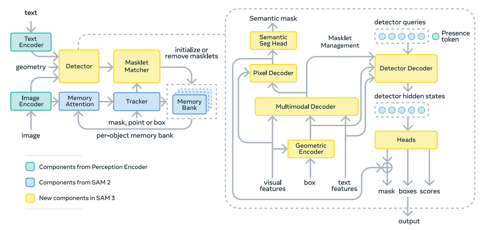
SAM 3 uses a dual encoder-decoder transformer architecture inspired by the earlier SAM models and by DETR. The goal is to support both Promptable Concept Segmentation (PCS) and Promptable Visual Segmentation (PVS), for images and videos, and for multiple prompt types such as concept prompts (simple noun phrases, image exemplars) or visual prompts (points, boxes, masks).

Image and Text Encoders

SAM 3 uses a vision encoder to extract image features and a text encoder to process the prompt. These encoder and decoders are Transformer-based and trained with contrastive vision–language learning on 5.4 billion image–text pairs through the Perception Encoder (PE). These encoders basic image features and text features that serve as inputs to the rest of the architecture.

Geometry and Exemplar Encoder

When prompts include visual examples, such as cropped objects, points or boxes, SAM 3 uses a geometry and exemplar encoder to turn them into learnable tokens using positional embeddings and ROI-pooled features. These tokens add visual and spatial information to the prompt.

Fusion Encoder

The text tokens and any geometry or exemplar tokens are combined into a single set of prompt tokens, which guide how the model interprets the image. The fusion encoder takes the unconditioned frame embeddings from the vision encoder and injects prompt information into them using six Transformer blocks with self-attention and cross-attention layers. This conditioning process effectively tells the model “what to look for,” resulting in conditioned frame embeddings that are aligned with the user’s prompt, whether it is text, visual examples or both.

Decoder

For prediction, SAM 3 uses a DETR style decoder with 200 learned object queries. Through six Transformer blocks, these queries self-attend and cross-attend to both the prompt tokens and the conditioned frame embeddings. The decoder includes improvements such as iterative box refinement, look-forward-twice, hybrid matching and Divide And Conquer (DAC) DETR. MLP heads applied to the queries output bounding boxes and scores, forming the base for instance-level predictions.

Presence Head

To improve classification accuracy, SAM 3 separates global classification from local localization. This head predicts whether the noun phrase is present in the image and helps separate global presence from local matching, reducing false positives.

Segmentation Head

Segmentation is handled by a MaskFormer style segmentation head that supports both semantic and instance segmentation. The conditioned frame embeddings generated by the fusion encoder are used to produce semantic masks, while the decoder’s object queries are used to generate instance masks. Because the vision encoder is a single-scale ViT, the segmentation head receives additional multi-scale features generated by a SimpleFPN module, enabling it to operate effectively across different spatial resolutions.

Ambiguity Head

Some noun phrases can refer to more than one visual concept, such as “apple” referring to either a fruit or a logo. Without special handling, the model might output conflicting or overlapping masks. To address this, SAM 3 uses a mixture-of-experts (MoE) ambiguity head with two experts trained in parallel using a winner-takes-all strategy, where only the expert with the lowest loss receives gradients. A small classification head learns to choose the correct expert at inference time. Additionally, overlapping instances are detected using Intersection-over-Minimum (IoM), which is more effective than IoU for nested objects, reducing ambiguous outputs by around 15%.

SAM 3 brings these components together into a unified system that can understand text and visual prompts, reason about object presence, and produce high-quality masks across images and videos. It expands segmentation beyond fixed category labels and make system more flexible, interactive and scalable.

SAM 3 Data and Training Infrastructure

The goal of SAM 3’s data and training system is to build a model that can segment any concept you name, not just a fixed list of object classes. To make this possible, the authors built two major pieces:

• A large-scale dataset called SA‑Co (Segment Anything with Concepts) covering millions of images, noun-phrases (concepts), and segmentation masks.
• A data engine that uses human and model in-loop annotation, to produce high quality data at large scale.

Let’s understand these.

SA-Co Dataset

The SA-Co (Segment Anything with Concepts) dataset forms the core training resource for SAM 3 and is designed to support large-scale, open-vocabulary concept segmentation across both images and videos. The data resource consists of training data and benchmark data.

SA-Co Training Data

Consists of three main image datasets and a video dataset:

• SA-Co/HQ: a high-quality collection produced through all stages of the data engine and containing 5.2 million images and 4 million unique noun phrases.
• SA-Co/SYN: a fully synthetic dataset labeled automatically by a mature version of the data engine.
• SA-Co/EXT: a group of fifteen external datasets enriched with additional noun-phrase labels and hard negatives using the SA-Co ontology.
• SA-Co/VIDEO: a video dataset with 52.5K videos, 24.8K unique phrases and 134K video-phrase pairs, with each video averaging 84 frames at 6 fps.

SA-Co Benchmark

For evaluation, the SA-Co Benchmark dataset is used which includes 214K unique phrases, 126K images and videos, and more than 3 million media-phrase pairs. The benchmark is divided into splits (Gold, Silver, Bronze, Bio and VEval) each differing in domain coverage and annotation depth, ranging from multi-annotator high-quality labels to masks generated using SAM 2.

• SA-Co/Gold: Covers 7 domains and provides three human annotations per pair for highest-quality evaluation.
• SA-Co/Silver: Includes 10 domains with one human annotation per image–phrase pair for scalable evaluation.
• SA-Co/Bronze and SA-Co/Bio: Includes 9 existing datasets either with existing mask annotations and masks generated by using boxes as prompts to SAM 2.
• SA-Co/VEval: A video benchmark spanning 3 domains, each with one annotation per video–phrase pair for temporal evaluation.

Data Engine

The SA-Co data engine is a large, human-model-in-the-loop system built to generate high-quality image and video annotations for training SAM 3. It combines captioning models, Llama-based AI verifiers, SAM models (SAM 1, SAM 2, SAM 3) and human annotators in a feedback loop. The core idea is straightforward:

• AI models propose concepts and masks
• humans and AI verifiers check them
• SAM 3 is retrained
• better annotations are produced in the next cycle

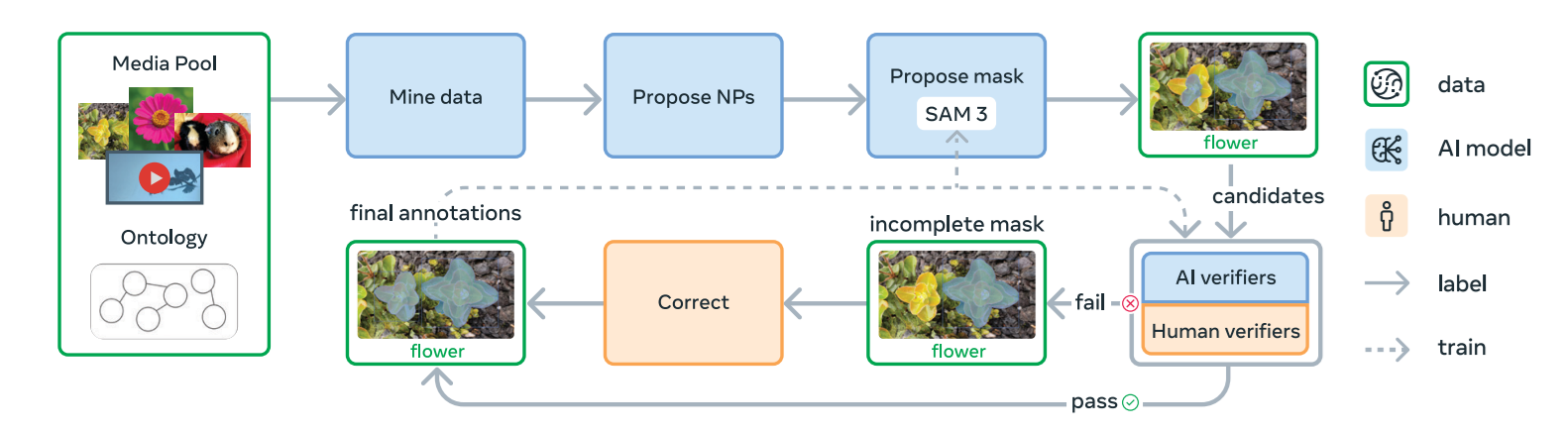
How the Data Engine Works (Components)

The engine begins by selecting images or videos from a large pool. A captioning model proposes noun phrases (NPs) that describe visual concepts in the media. A segmentation model (SAM 2 in Phase 1, and SAM 3 from Phase 2 onward) then generates candidate masks for each phrase.

These masks go through two human or AI-assisted checks:

• Mask Verification (MV): Annotators decide whether the mask is correct for the phrase.
• Exhaustivity Verification (EV): Annotators check if all instances of that concept have been masked.

If the result is incomplete, it goes to manual correction, where humans add, remove or adjust masks using a browser-based tool powered by SAM 1. Annotators may also use “group masks” for small objects or reject phrases that cannot be grounded.

The Four Phases of the Data Engine

Following are the four phases of data engine.

Phase 1: Human Verification

In the first phase, images are sampled randomly and a simple captioning model proposes noun phrases for each one. SAM 2 is used to generate candidate masks, and humans verify every mask for both quality and correctness. This phase produces 4.3 million image–phrase pairs, which serve as the initial training data for SAM 3.

Phase 2: Human + AI Verification

In Phase 2, the human annotations collected earlier are used to train Llama 3.2-based AI verifiers, which can automatically evaluate mask quality and exhaustiveness. The noun-phrase generator is upgraded to a Llama-based system, and SAM 3 replaces SAM 2 as the mask-proposal model. With humans now focused only on difficult cases, the pipeline becomes much faster and produces 122 million new image–phrase pairs.

Phase 3: Scaling and Domain Expansion

Phase 3 expands the dataset by having AI models mine harder examples across 15 different domains. New concepts are added by extracting noun phrases from image alt-text and from a large 22.4M-node Wikidata-based ontology. During this phase, SAM 3 and the AI verifiers are retrained multiple times, resulting in 19.5 million additional pairs and much broader concept coverage.

Phase 4: Video Annotation

The final phase extends the data engine from images to videos. A video-enabled version of SAM 3 generates masklets across frames, while the mining process focuses on challenging clips with crowding or tracking failures. Human effort is directed toward these difficult cases, ultimately producing 52.5K annotated videos and 467K masklets.

The data engine continuously improves itself through a cycle of AI proposals, human feedback and model retraining. Over four phases, it scales up in both complexity and automation, allowing SA-Co to grow in size, variety and quality. By combining captioning models, Llama-based AI verifiers and multiple generations of SAM, the engine produces the massive open-vocabulary dataset needed to train SAM 3.

Promptable Concept Segmentation Conclusion

Promptable Concept Segmentation changes the way we think about segmentation. Instead of choosing from a fixed set of labels, we can now describe what we want in natural language and let the model find it. SAM 3 shows how powerful this can be by handling flexible prompts, understanding complex concepts and segmenting them across images and video. SAM 3 with PCS proves that interacting with vision models will feel more natural, more open-ended and much closer to how we describe things in everyday life.

Cite this Post

Use the following entry to cite this post in your research:

Timothy M. (Nov 19, 2025). What Is Promptable Concept Segmentation (PCS)?. Roboflow Blog: https://blog.roboflow.com/what-is-promptable-concept-segmentation-pcs/