
Basketball is one of the hardest sports for computer vision. Players move at high speed, causing motion blur. Bodies crash into each other and overlap, making jersey numbers hard to see. Uniforms look almost identical, so appearance alone is not enough to tell players apart. On top of that, the camera keeps zooming and panning, changing perspective every second.
In this blogpost, we show how to overcome these challenges and build a computer vision system that can detect, track, and recognize NBA players during a game.
We open-sourced the basketball player recognition code!
Models
Reliable player identification is hard. You must first detect the player, track them consistently across all frames, and then accurately read the small, often obscured number on their jersey. This complex task requires combining multiple state-of-the-art computer vision models into a single, robust pipeline.
- RF-DETR: A state-of-the-art object detection model. It is both fast and accurate. We use it to detect players, jersey numbers, and basketball objects like the ball and rim.
- SAM2 (Segment Anything Model 2): A unified model for object segmentation and tracking in both images and videos. You prompt SAM2 with points or bounding boxes to select an object. It then tracks and segments that object across video frames.
- SmolVLM2: A compact vision-language model specialized in image-to-text tasks. We rely on it for Optical Character Recognition (OCR) of cropped jersey numbers.
- ResNet: A well-known Convolutional Neural Network. We fine-tuned it to classify crops of jersey numbers.
- SigLIP: A vision-language model similar to CLIP, optimized for image-text alignment. We use SigLIP to generate embeddings that capture visual similarity, which enables robust team clustering.
- K-means: A simple, yet highly effective, clustering algorithm. K-means partitions data points into a predefined number of clusters. We apply it to separate players into teams based on their SigLIP embeddings.
Detect Players with RF-DETR
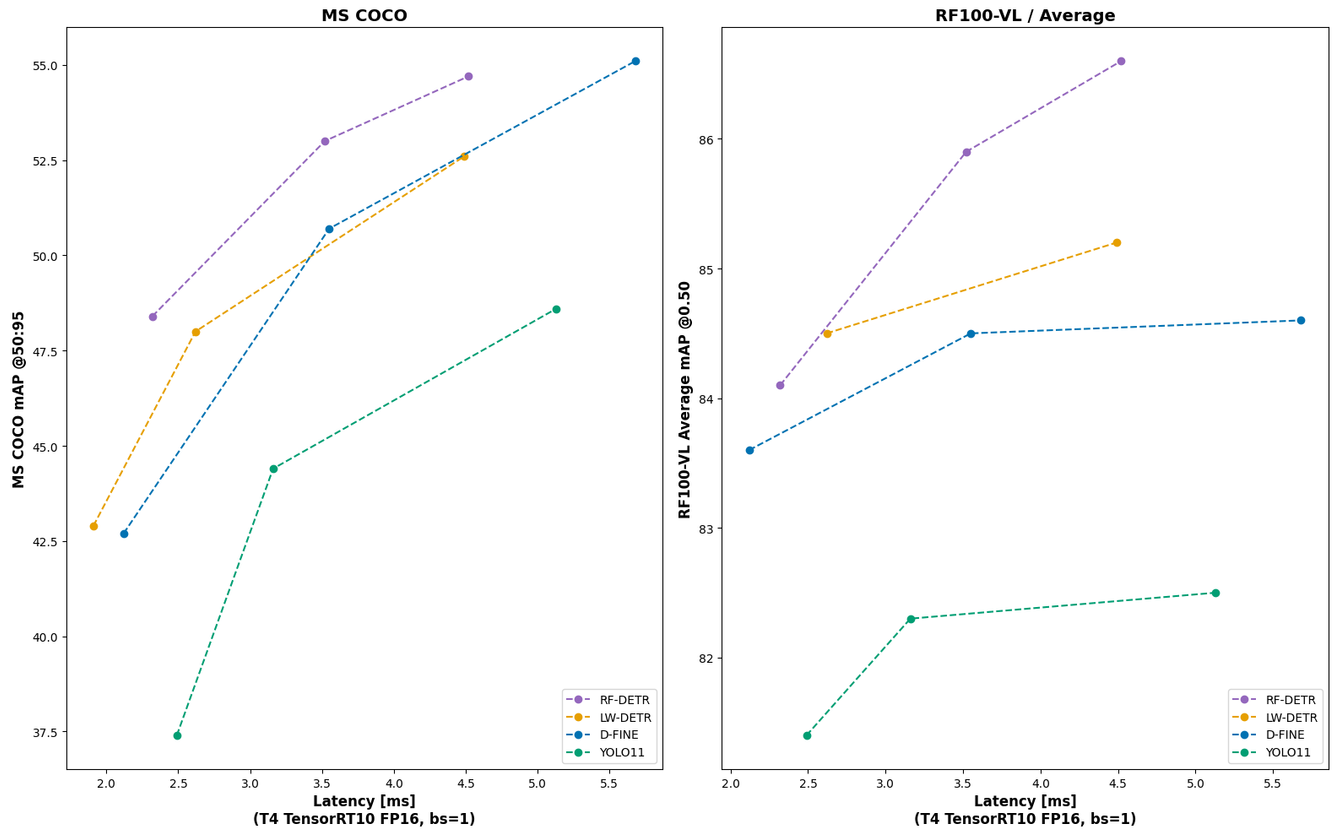
The first step is object detection. We use RF-DETR-S because it offers the best balance of speed and accuracy for our task. On the COCO benchmark, RF-DETR-S outperforms larger models like YOLO11-L while running faster, and its strong generalization makes it reliable for basketball scenes with motion blur, overlaps, and small jersey numbers.
We fine-tuned RF-DETR on a custom dataset with 10 classes: ball, ball-in-basket, number, player, player-in-possession, player-jump-shot, player-layup-dunk, player-shot-block, referee, and rim.
For player recognition, we rely on the number class together with all player-related classes (such as player, player-in-possession, player-jump-shot, player-layup-dunk, and player-shot-block). The remaining classes are not needed here but are useful for other tasks like detecting shots and judging whether a basket was made, which we will cover in a separate tutorial.
Example of RF-DETR detecting jump shots and classifying shot outcomes.
The model was trained for free on the Roboflow platform. You can also fine-tune it yourself, either locally or in Google Colab. A full tutorial is available on our YouTube channel.
YouTube walkthrough on fine-tuning RF-DETR on a custom dataset.
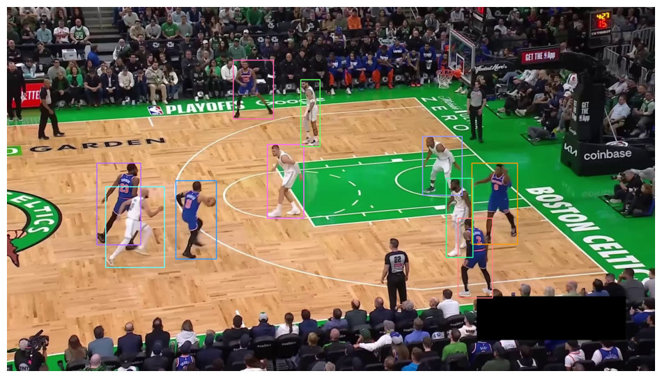
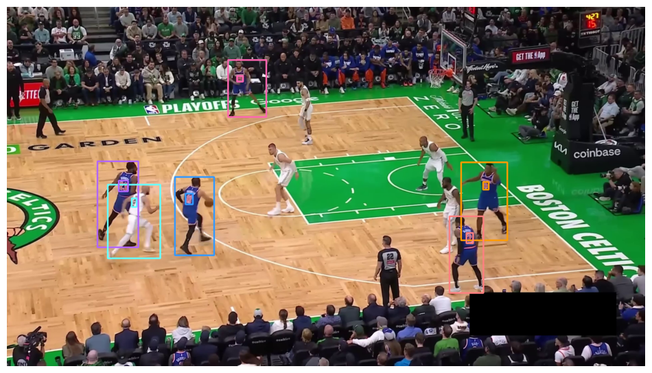
RF-DETR detecting players and jersey numbers in game footage.
Track Players with SAM2
The next step is tracking. We use SAM2, which is designed for segmentation and tracking in videos. SAM2 has an internal memory mechanism (often called a ”temporal memory bank”) that stores the appearance of each object over time. This mechanism makes the model robust to occlusion. When a player is blocked and disappears from view, SAM2 uses the stored features to re-identify and continue tracking them once they reappear.
SAM2 Prompting
We start by running RF-DETR on the first frame of a video to detect all players. The bounding boxes from RF-DETR are then used as prompts for SAM2. From that point, SAM2 segments and tracks the players across the clip.
In our experiments, we work with short video clips where all players are visible in the first frame. For longer clips, it would be necessary to add a component that monitors detections and re-prompts SAM2 to make sure every player stays tracked throughout the sequence.
Cleaning Up SAM2 Tracking Errors
Processing high-action basketball videos sometimes causes SAM2 to make errors. These errors often result in a mask that consists of multiple disconnected segments with large distances between them. For instance, after a shot or pass, SAM2 might incorrectly classify the ball or a background element as part of the player’s mask. We must clean these errors before proceeding.
Example of SAM2 tracking before (left) and after (right) applying mask cleanup.
Our cleanup function addresses these multi-segment masks. It finds all segments within the binary mask, identifies the largest segment as the main player body, and removes any other smaller segments whose center is beyond a set distance threshold from the main segment’s center.
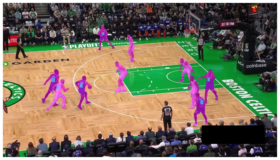
SAM2 tracking players across a video clip, with IDs maintained through occlusions.
Unsupervised Team Clustering with SigLIP, UMAP and K-means
Every basketball game has different uniforms and court conditions. To create a generalized solution that works across different games without manual data annotation, we used an unsupervised learning strategy to separate players into their respective teams.
Generating Player Embeddings
The first step is to build our training set by going through all sample videos from our selected game. We extract one frame per second and run player detection on it using our fine-tuned RF-DETR-S model. From each detection we crop the player region, then use SigLIP to generate embeddings for every crop.
SigLIP is a vision-language model trained on large-scale image–text pairs. It works similarly to CLIP but uses a sigmoid loss instead of softmax, which improves training stability and performance. The model outputs high-dimensional embeddings that capture both low-level visual cues like color and texture, and higher-level semantic information. This makes it well-suited for measuring player similarity based on uniforms, even when lighting or camera angles change.
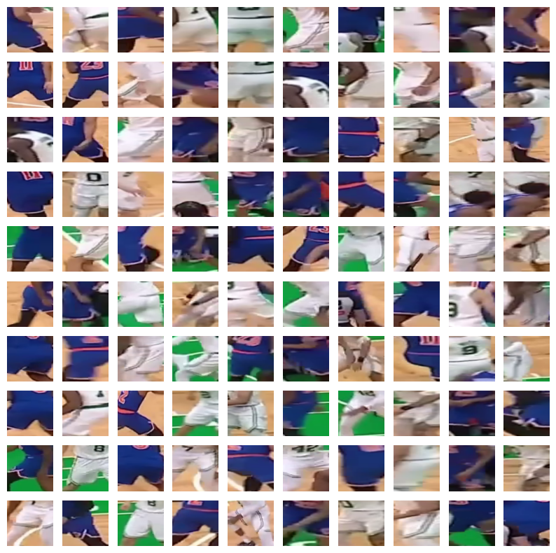
It is important to note that we do not use the full detection bounding box for cropping. Instead, we take only the central part of the box. Depending on the player’s pose and location on the court, the bounding box may include a lot of noise, such as players from the opposing team or the crowd, which could harm the clustering results. The central crop usually contains the most relevant information about the player we want to track.
Dimensionality Reduction and Clustering
The resulting SigLIP embeddings are high-dimensional. We use UMAP (Uniform Manifold Approximation and Projection) to reduce these to three dimensions. UMAP is a popular choice for dimensionality reduction because it preserves both the local and global structure of the data, which is crucial for subsequent clustering.
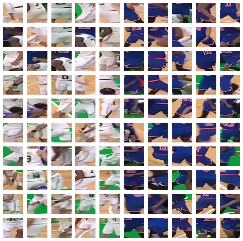
Finally, we apply K-means clustering, a simple yet effective algorithm, to partition the data into two groups. If the process works as expected, the crops separate into two distinct clusters, with each cluster representing one team based on the uniform’s visual features. We used a similar approach in our Football AI project. Watch our YouTube tutorial to learn more.
YouTube tutorial explaining team clustering in detail, first applied in our Football AI project.
Players grouped into two clusters representing each team based on uniform features.
Identifying Player Numbers
With players tracked and teams identified, the final step is to read the number on the jersey and pair it with the correct player.
Number OCR with SmolVLM2
We first experimented with SmolVLM2, a compact vision-language model. With its small size, SmolVLM2 is powerful and fast, which made the model an attractive choice for OCR in our pipeline. SmolVLM2 was pre-trained mainly on document OCR, but it transferred surprisingly well to jersey numbers in basketball. Out of the box, it reached 56% accuracy on our test set. This was not high enough for reliable player recognition. The model also sometimes produced implausible predictions in a basketball context, such as “011” or “3000.”
To improve performance, we fine-tuned SmolVLM2 on a custom dataset of jersey number crops collected from the 2025 NBA Playoffs. The dataset contained 3.6k images.
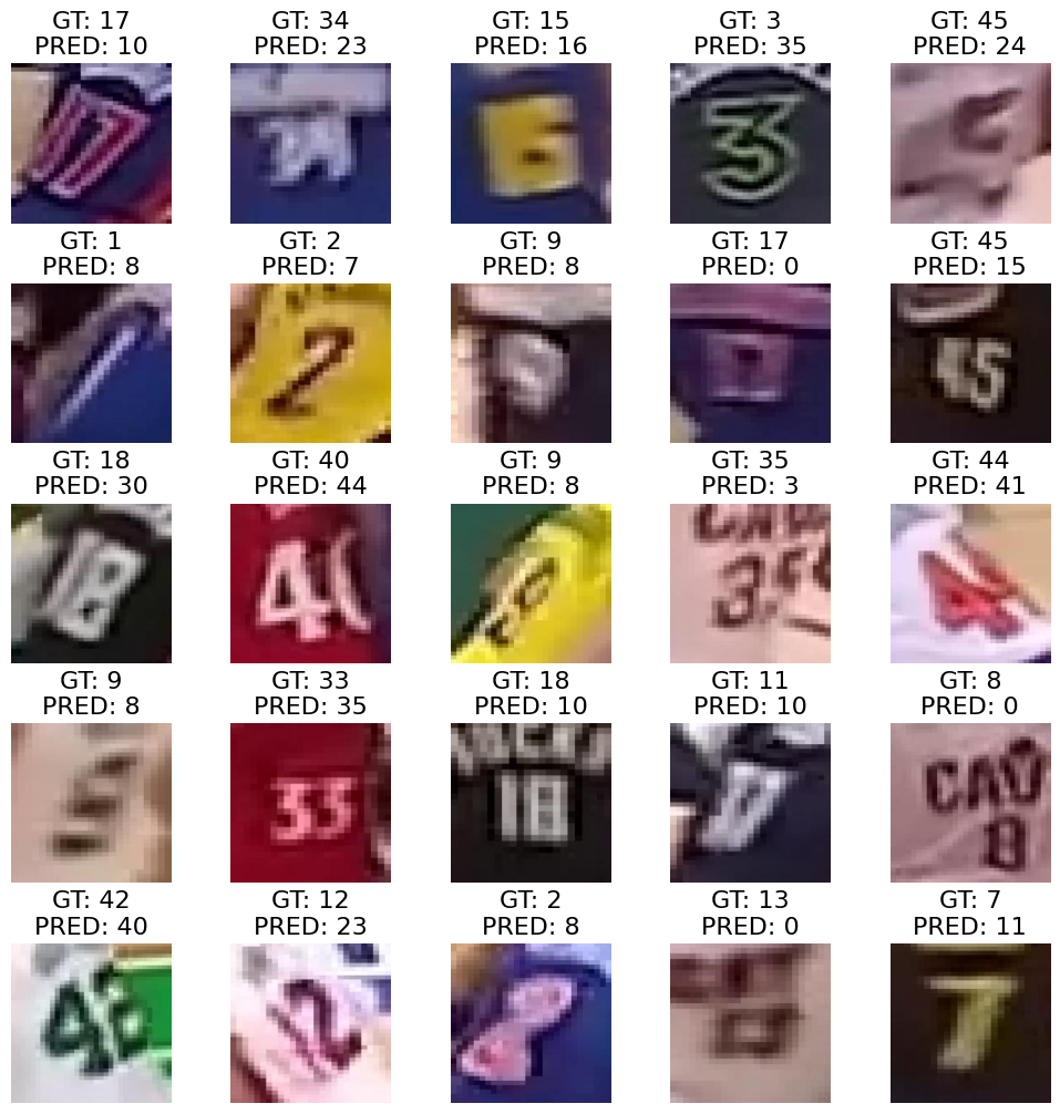
Numbers were first auto-annotated with a pre-trained SmolVLM2 model, then manually refined. The dataset is relatively large but incomplete (some numbers between 00 and 99 are missing) and imbalanced. For example, “8” appears 315 times (8.7%), while “6” appears only 8 times (0.2%). This imbalance reflects the real distribution of numbers on the court. After fine-tuning, SmolVLM2 improved to 86% accuracy on the test set.
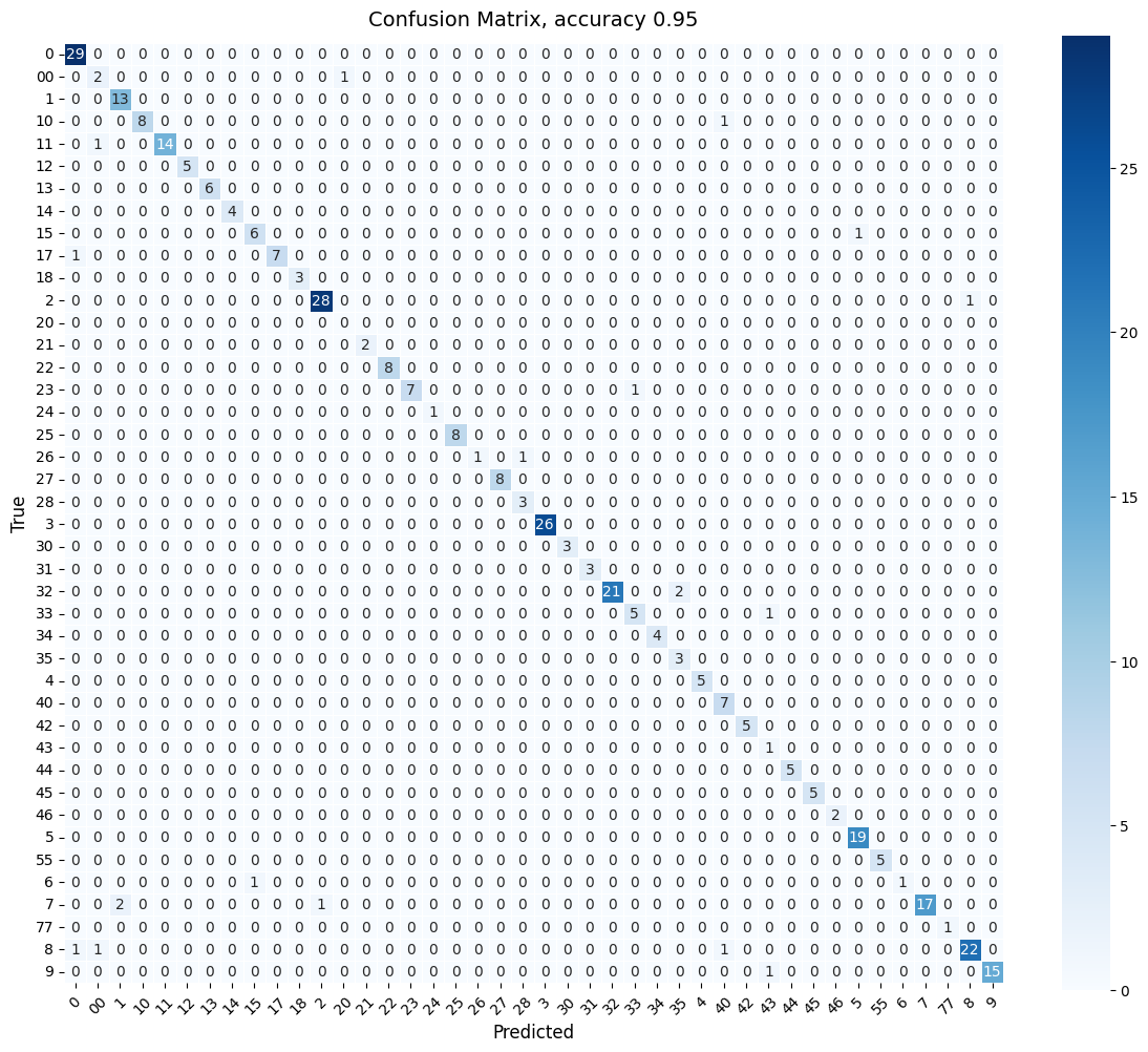
Number Classification with ResNet
We also tested a simpler approach with a classification model. We fine-tuned a ResNet-32 on the same dataset, which was reformatted from JSONL into a directory-structured dataset typical for image classification. ResNet reached 93% accuracy on the test set, outperforming the fine-tuned SmolVLM2. This shows that a lightweight CNN trained specifically for number classification can be more effective than a general-purpose VLM, even a strong one like SmolVLM2.
Pairing Numbers to Players with IoS
Once jersey numbers are detected, the next step is to assign them to the correct player. The challenge is that player masks from SAM2 and number detections from RF-DETR are separate outputs. We need a reliable way to match them.
We use the Intersection over Smaller Area (IoS) metric. IoS is similar to IoU (Intersection over Union) but normalizes by the smaller region. Since a jersey number is always smaller than a player mask, IoS measures how much of the number is contained within the player. An IoS of 1.0 means the number is fully inside the player mask. We keep only matches with IoS ≥ 0.9. To do this, we use SAM2 masks for players and convert RF-DETR number bounding boxes into masks before computing IoS.
Resolving Player Identity
Even with 93% test accuracy, recognition is not perfect. Errors occur most often when players are far from the camera, such as spot-up shooters waiting in the corner. To improve reliability, we do not rely on a single prediction. Instead, we sample numbers every 5 frames. This interval is long enough for players to change pose and camera angle, but short enough to collect multiple predictions for each player.
Impact of player position on jersey number visibility.
We then apply a simple heuristic: a jersey number is confirmed once the same prediction appears three times in a row. This stabilizes recognition without adding complexity. Accuracy can be improved further if we constrain predictions to the set of numbers known to be on the court at a given time. The final step is to map each confirmed number and team to a player’s name from the roster.
End-to-end system result showing detection, tracking, and player recognition in action.
Conclusions
Building a system to detect, track, and identify basketball players is challenging. Motion blur, occlusion, and uniform similarity make it a difficult problem for computer vision. In this post, we showed how to overcome these challenges with a pipeline that combines state-of-the-art models: RF-DETR for detection, SAM2 for tracking, SigLIP with UMAP and K-means for team clustering, and SmolVLM2 with ResNet for jersey number recognition.
This pipeline is not real-time. On an NVIDIA T4 it runs at around 1–2 FPS. The goal of this project was not to achieve production speed but to test what is possible with today’s models. The biggest source of slowdown is SAM2. While it is a real-time tracker, its performance drops as the number of tracked objects increases. You can improve throughput by lowering video resolution, using a smaller SAM2 checkpoint, or distilling SAM2 basketball knowledge into a lighter model.
The result is a working system that can follow every player on the court and resolve their identity during live gameplay. While there is room for improvement, especially in number recognition under difficult conditions, this approach demonstrates how modern computer vision models can be combined to solve real-world sports analytics tasks.
We open-sourced the full code so you can try it yourself, experiment with different models, and extend the pipeline further.
Cite this Post
Use the following entry to cite this post in your research:
Piotr Skalski. (Sep 30, 2025). How to Detect, Track, and Identify Basketball Players with Computer Vision. Roboflow Blog: https://blog.roboflow.com/identify-basketball-players/