
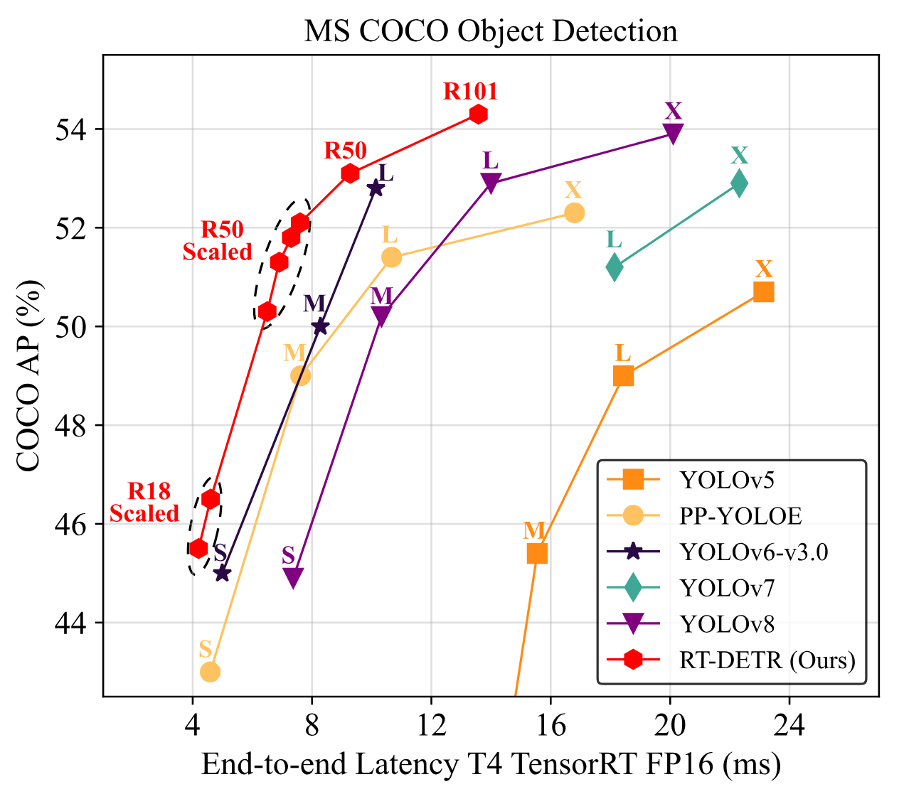
RT-DETR, short for "Real-Time DEtection TRansformer", is a computer vision model developed by Peking University and Baidu. In their paper, "DETRs Beat YOLOs on Real-time Object Detection" the authors claim that RT-DETR can outperform YOLO models in object detection, both in speed and accuracy. The model has been released under the Apache 2.0 license, making it a great option, especially for enterprise projects.
Recently, RT-DETR was added to the `transformers` library, significantly simplifying its fine-tuning process. In this tutorial, we will show you how to train RT-DETR on a custom dataset. Go here to immediately access the Colab Notebook. Let's dive in!
Overview of RT-DETR
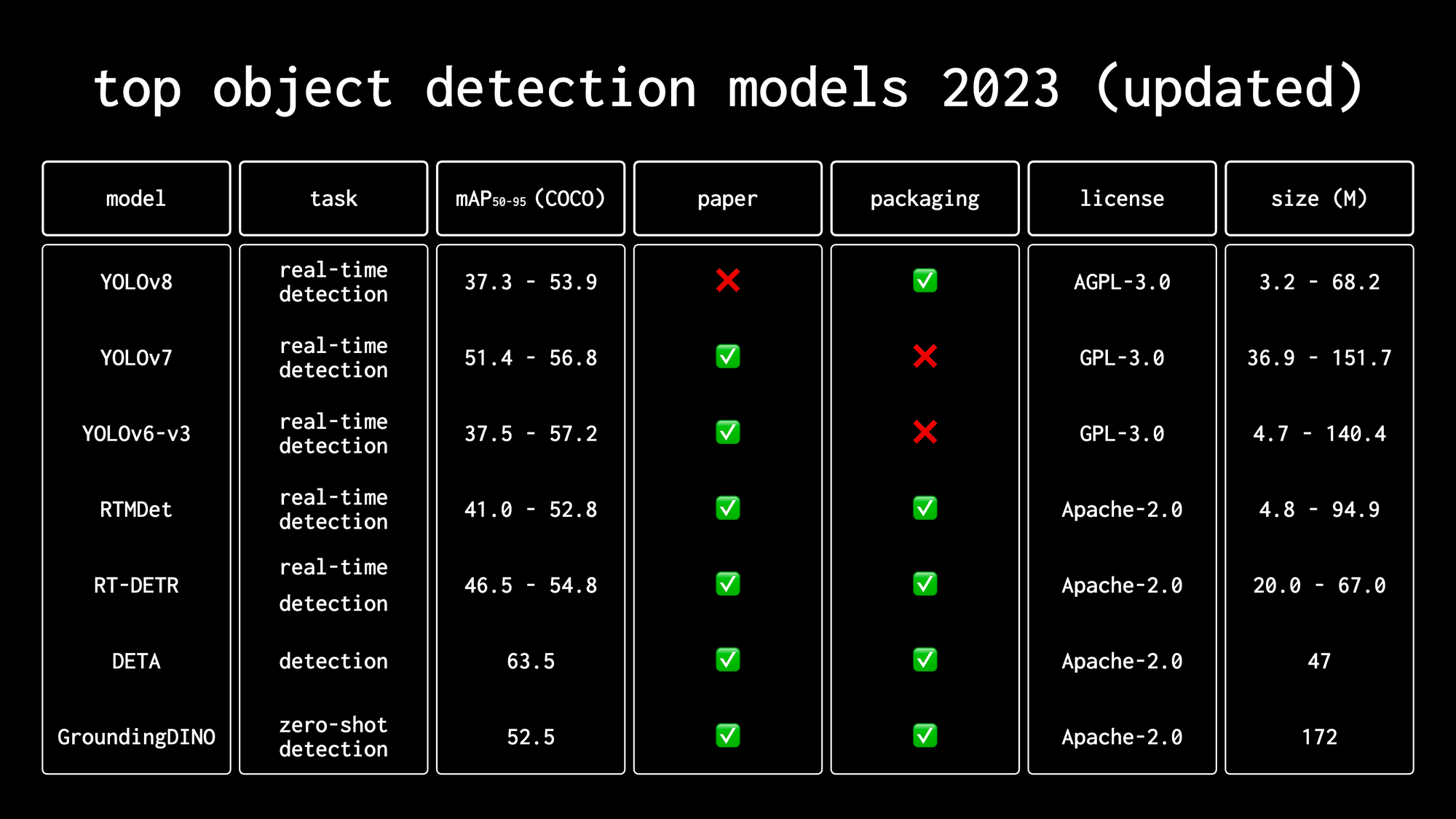
We mentioned RT-DETR in our video, "Top Object Detection Models in 2023". Check it out if you want to see a comparison of RT-DETR with other popular object detection models like different versions of YOLO, RTMDet, or GroundingDINO.
RT-DETR builds upon the DETR model developed by Meta AI in 2020, which was the first to successfully leverage the transformer architecture for object detection. DETR revolutionized object detection by eliminating the need for hand-designed components like non-maximum suppression and anchor generation, streamlining the detection pipeline.
Before you start
To train RT-DETR on a custom dataset, we need to properly configure our environment. This tutorial is accompanied by a notebook that you can open in a separate tab and follow along.
GPU Acceleration
If you are using our Google Colab, ensure you have access to an NVIDIA T4 GPU by running the nvidia-smi command. If you encounter any issues, navigate to Edit -> Notebook settings -> Hardware accelerator, set it to T4 GPU, and then click Save.
If you are running the code locally, you will also need an NVIDIA GPU with approximately 11GB VRAM assuming a batch size of 16. Depending on the amount of memory on your GPU, you may need to choose different hyperparameter values during training.
Secrets
Additionally, we will need to set the values of two secrets: the HuggingFace token, to download the pre-trained model, and the Roboflow API key, to download the object detection dataset.
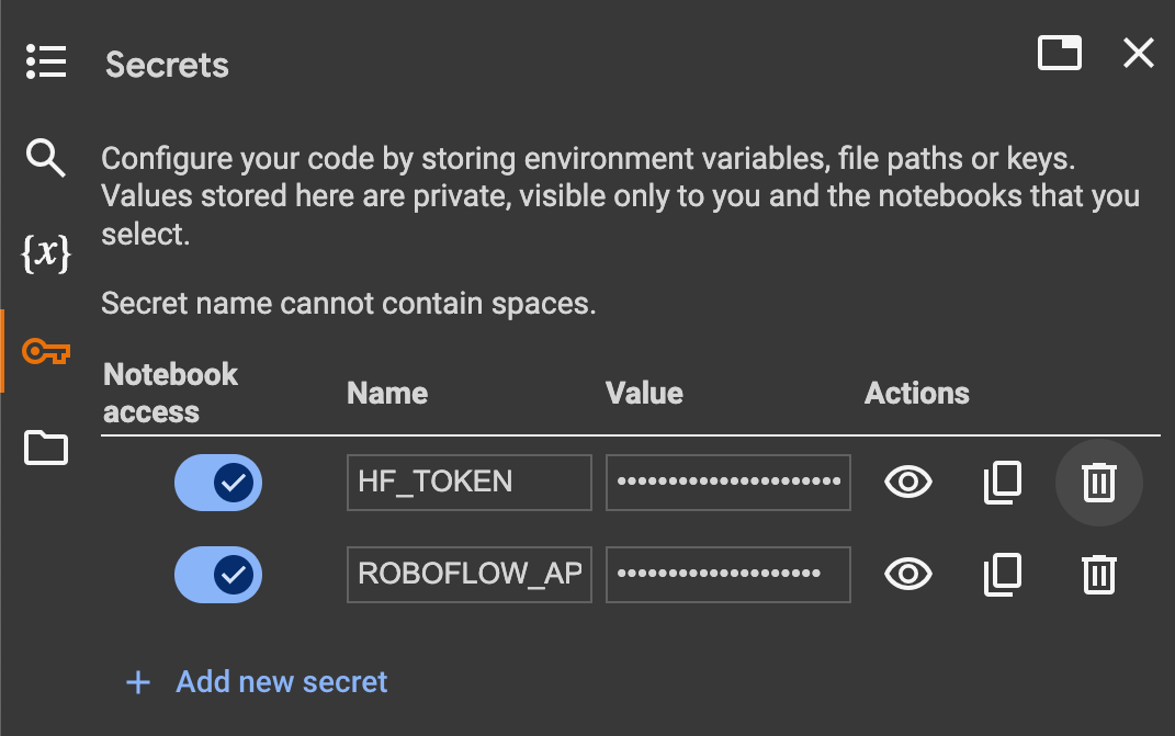
Open your HuggingFace settings page, clickAccess Tokens, then New Token to generate a new token. To get the Roboflow API key, go to your Roboflow settings page, click Copy. This will place your private key in the clipboard. If you are using Google Colab, go to the left pane and click on Secrets (🔑).
Then store the HuggingFace Access Token under the name HF_TOKEN and store the Roboflow API Key under the name ROBOFLOW_API_KEY. If you are running the code locally, simply export the values of these secrets as environment variables.
The last step before we begin is to install all the necessary dependencies. We will need transformers and accelerate to train the model, roboflow to download the dataset from Roboflow Universe, albumentations and supervision to augment our dataset and feed it to our model during training. Finally, we'll use torchmetrics to benchmark the model and measure its performance on the validation dataset during training.
pip install -q git+https://github.com/huggingface/transformers.git
pip install -q git+https://github.com/roboflow/supervision.git
pip install -q accelerate roboflow torchmetrics
pip install -q "albumentations>=1.4.5"
Load pre-trained RT-DETR model
Before we start, let's load our pre-trained model into memory and perform a test inference. This is one of the easiest ways to confirm that our environment is set up correctly and everything is working as expected.
We choose the checkpoint we want to use and then initialize the model and processor. In the transformers library, the model encapsulates the architecture and learned parameters, while the processor handles the preprocessing of input data (images in our case) and postprocessing of model outputs to obtain the final predictions.
import torch
from transformers import AutoModelForObjectDetection, AutoImageProcessor

CHECKPOINT = "PekingU/rtdetr_r50vd_coco_o365"
DEVICE = torch.device("cuda" if torch.cuda.is_available() else "cpu")

model = AutoModelForObjectDetection.from_pretrained(CHECKPOINT).to(DEVICE)
processor = AutoImageProcessor.from_pretrained(CHECKPOINT)
To perform inference, we load our image using the Pillow library - it is available out of the box in Google Colab, but if you are running the code locally you will also need to install it separately.
Next, we pass it through the processor, which performs normalization and resizing of the image. The prepared input is then passed through the model. It is important to note that the inference is enclosed within the torch.no_grad context manager.
This context manager temporarily disables gradient calculations, which is essential for inference as it reduces memory consumption and speeds up computations since gradients are not needed during this phase.
import requests
from PIL import Image

URL = "https://media.roboflow.com/notebooks/examples/dog.jpeg"

image = Image.open(requests.get(URL, stream=True).raw)
inputs = processor(image, return_tensors="pt").to(DEVICE)

with torch.no_grad():
    outputs = model(**inputs)

w, h = image.size
results = processor.post_process_object_detection(
    outputs, target_sizes=[(h, w)], threshold=0.3)
The easiest way to visualize the results of RT-DETR, as well as any object detection and segmentation model in the transformers library is to use the from_transformers connector available in the supervision package. It allows you to convert the raw model output to the common sv.Detections format.
Now you can take advantage of a wide range of annotators and tools available in supervision. You can also easily apply non-max suppression (NMS).
detections = sv.Detections.from_transformers(results[0]).with_nms(threshold=0.1)
labels = [
    model.config.id2label[class_id]
    for class_id
    in detections.class_id
]

annotated_image = image.copy()
annotated_image = sv.BoundingBoxAnnotator().annotate(
    annotated_image, detections)
annotated_image = sv.LabelAnnotator().annotate(
    annotated_image, detections, labels=labels)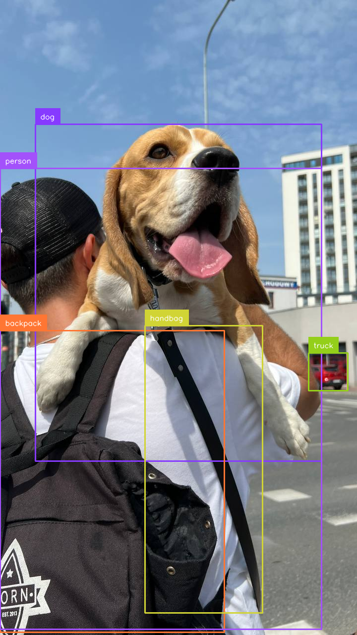
Prepare Dataset for Training RT-DETR
Download the dataset from Roboflow Universe
To train RT-DETR, you will need an object detection dataset. For this tutorial, we will use a dataset in COCO format. You can easily use datasets in PASCAL VOC and YOLO formats by making minimal changes to the code, which I will mention shortly.
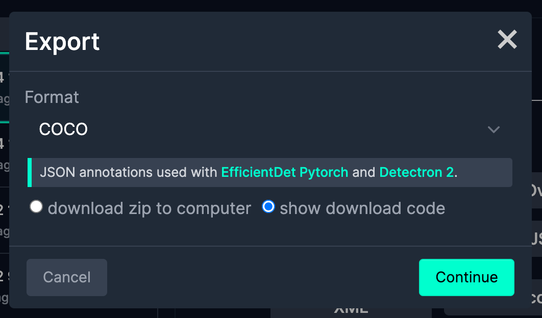
To download a dataset from Roboflow Universe, click the `Export Dataset` button, and when the popup opens, select your desired output format from the dropdown - in our case, COCO. Also, check the "Show download code" option. After a few seconds, a code snippet will be generated that you can copy into your Google Colab notebook or training script.
from roboflow import Roboflow
from google.colab import userdata

ROBOFLOW_API_KEY = userdata.get('ROBOFLOW_API_KEY')
rf = Roboflow(api_key=ROBOFLOW_API_KEY)

project = rf.workspace("roboflow-jvuqo").project("poker-cards-fmjio")
version = project.version(4)
dataset = version.download("coco")
Load Dataset
Once we have the dataset on disk, it's time to load it into memory. The supervision package offers easy-to-use DetectionDataset utilities that allow you to easily load annotations in various formats.
In our case, we usefrom_coco, but from_pascal_voc and from_yolo are also available, as you can read in the documentation. `DetectionDataset` also allows you to easily split, merge, and filter detection datasets. It also easily integrates with PyTorchDataset, which you will see shortly. PyTorch Dataset is an abstract class that provides a convenient way to access and process data samples in a standardized format, making it a fundamental building block for training machine learning models.
ds_train = sv.DetectionDataset.from_coco(
    images_directory_path=f"{dataset.location}/train",
    annotations_path=f"{dataset.location}/train/_annotations.coco.json",
)
ds_valid = sv.DetectionDataset.from_coco(
    images_directory_path=f"{dataset.location}/valid",
    annotations_path=f"{dataset.location}/valid/_annotations.coco.json",
)
ds_test = sv.DetectionDataset.from_coco(
    images_directory_path=f"{dataset.location}/test",
    annotations_path=f"{dataset.location}/test/_annotations.coco.json",
)
Data Augmentations for Training RT-DETR
Data augmentation is one of the simplest ways to improve the accuracy of a fine-tuned model. In computer vision projects, data augmentation involves applying various transformations to the training images, such as rotations, flips, crops, and color adjustments. This technique artificially increases the size and diversity of the training dataset, helping the model generalize better and become more robust to variations in real-world data.
A popular way to apply augmentation is to use the albumentations package. The first step is to define the transformations we want to apply. Albumentations offers dozens of them, but for the purposes of this tutorial, we will only use four.
import albumentations as A
augmentation_train = A.Compose(
[
A.Perspective(p=0.1),
A.HorizontalFlip(p=0.5),
A.RandomBrightnessContrast(p=0.5),
A.HueSaturationValue(p=0.1),
],
bbox_params=A.BboxParams(
format="pascal_voc",
label_fields=["category"],
clip=True,
min_area=25
),
)
augmentation_valid = A.Compose(
[A.NoOp()],
bbox_params=A.BboxParams(
format="pascal_voc",
label_fields=["category"],
clip=True,
min_area=1
),
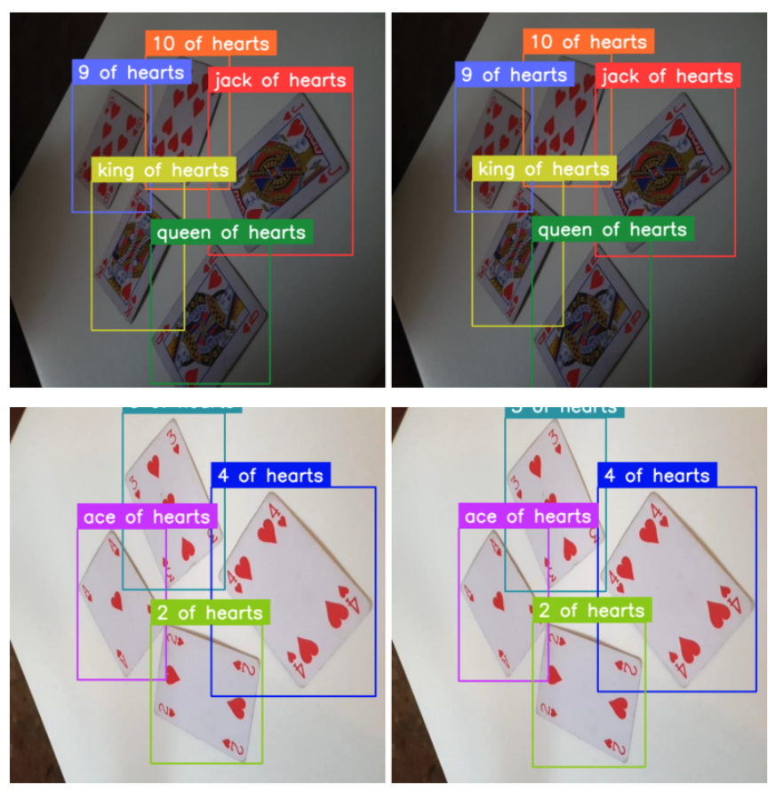
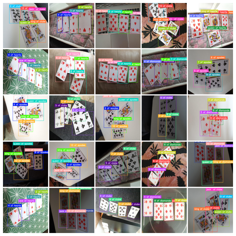
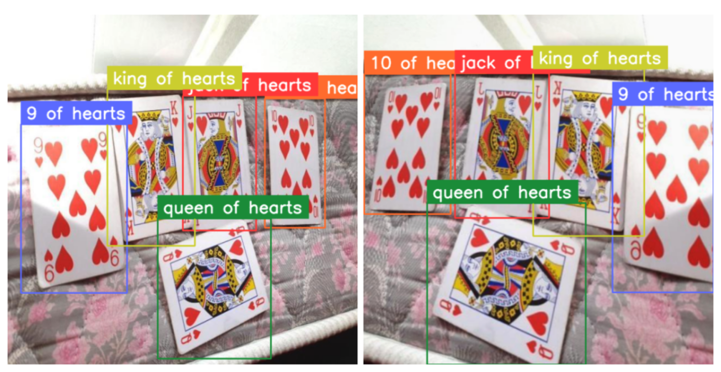
)Now we can easily apply these transformations to the supervision DetectionDataset entries. Here is a comparison of a few pairs - original and augmented images.
from dataclasses import replace

IMAGE_COUNT = 5

for i in range(IMAGE_COUNT):
    _, image, annotations = ds_train[i]

    output = augmentation_train(
        image=image,
        bboxes=annotations.xyxy,
        category=annotations.class_id
    )

    augmented_image = output["image"]
    augmented_annotations = replace(
        annotations,
        xyxy=np.array(output["bboxes"]),
        class_id=np.array(output["category"])
    )
Define PyTorch Dataset
The processor expects the annotations to be in the following format: {'image_id': int, 'annotations': List[Dict]}, where each dictionary is a COCO object annotation. Let's define a PyTorch Dataset that will load annotations from disk, augment them, and return them in the format expected by the RT-DETR processor. The following code snippet may look intimidating, but if we look closer, there is nothing new here except for the conversion of annotations to COCO format.
class AugmentedDetectionDataset(Dataset):
    def __init__(self, dataset, processor, transform):
        self.dataset = dataset
        self.processor = processor
        self.transform = transform

    @staticmethod
    def annotations_as_coco(image_id, categories, boxes):
        ...

    def __len__(self):
        return len(self.dataset)

    def __getitem__(self, idx):
        _, image, annotations = self.dataset[idx]

        image = image[:, :, ::-1]
        transformed = self.transform(
            image=image,
            bboxes=annotations.xyxy,
            category=annotations.class_id
        )
        image = transformed["image"]
        boxes = transformed["bboxes"]
        categories = transformed["category"]

        formatted_annotations = self.annotations_as_coco(
            image_id=idx,
            categories=categories,
            boxes=boxes
        )
        result = self.processor(
            images=image,
            annotations=formatted_annotations,
            return_tensors="pt"
        )

        return {k: v[0] for k, v in result.items()}
Now all we have to do is initialize the datasets for the train, test, and valid subsets. Pay attention to applying different augmentations for the training set and different ones for the validation and test sets.
augmented_dataset_train = AugmentedDetectionDataset(
    ds_train, processor, transform=augmentation_train)
augmented_dataset_valid = AugmentedDetectionDataset(
    ds_valid, processor, transform=augmentation_valid)
augmented_dataset_test = AugmentedDetectionDataset(
    ds_test, processor, transform=augmentation_valid)
The last thing we need to do is define the collect_fn callback. In PyTorch, the collect_fn is a function that is passed to the DataLoader to customize how the individual data samples are collated into a batch. In our case, we need it to pad the images and labels to the same size, as the RT-DETR model expects a fixed-size input.
def collate_fn(batch):
    data = {}
    data["pixel_values"] = torch.stack([
        x["pixel_values"]
        for x
        in batch]
    )
    data["labels"] = [x["labels"] for x in batch]
    return data
Fine-tuning RT-DETR - Code Overview
Most of the heavy lifting is behind us, and we are now ready to train the model. Let's start by loading the model with AutoModelForObjectDetection using the same checkpoint as in the preprocessing step.
id2label = {id: label for id, label in enumerate(ds_train.classes)}
label2id = {label: id for id, label in enumerate(ds_train.classes)}

model = AutoModelForObjectDetection.from_pretrained(
    CHECKPOINT,
    id2label=id2label,
    label2id=label2id,
    anchor_image_size=None,
    ignore_mismatched_sizes=True,
)
In the TrainingArguments use output_dir to specify where to save your model, then configure hyperparameters as you see fit. For num_train_epochs=20 training will take about 30 minutes in Google Colab T4 GPU, increase the number of epochs to get better results.
training_args = TrainingArguments(
    output_dir=f"{dataset.name.replace(' ', '-')}-finetune",
    num_train_epochs=20,
    max_grad_norm=0.1,
    learning_rate=5e-5,
    warmup_steps=300,
    per_device_train_batch_size=16,
    dataloader_num_workers=2,
    metric_for_best_model="eval_map",
    greater_is_better=True,
    load_best_model_at_end=True,
    eval_strategy="epoch",
    save_strategy="epoch",
    save_total_limit=2,
    remove_unused_columns=False,
    eval_do_concat_batches=False,
)
Finally, we are ready to start training. All we need to do is pass the training arguments to the Trainer along with the model, dataset, image processor, and data collator. The Trainer class orchestrates the entire training process, handling optimization, evaluation, and checkpointing.
trainer = Trainer(
    model=model,
    args=training_args,
    train_dataset=pytorch_dataset_train,
    eval_dataset=pytorch_dataset_valid,
    tokenizer=processor,
    data_collator=collate_fn,
    compute_metrics=eval_compute_metrics_fn,
)

trainer.train()
Trained RT-DETR Model Evaluation
Once the training is complete, it's time to benchmark our model on the test subset. We begin by collecting two lists: target annotations and model predictions. To do this, we loop over our test dataset and perform inference using our newly trained model.
import supervision as sv

targets = []
predictions = []

for i in range(len(ds_test)):
    path, sourece_image, annotations = ds_test[i]

    image = Image.open(path)
    inputs = processor(image, return_tensors="pt").to(DEVICE)

    with torch.no_grad():
        outputs = model(**inputs)

    w, h = image.size
    results = processor.post_process_object_detection(
        outputs, target_sizes=[(h, w)], threshold=0.3)

    detections = sv.Detections.from_transformers(results[0])

    targets.append(annotations)
    predictions.append(detections)
Mean Average Precision (mAP) is a widely used metric for evaluating object detection models. It considers both the accuracy of object localization (bounding boxes) and classification, providing a single comprehensive performance measure. Calculating mAP using the supervision package is very simple. As a result, our model achieved almost 0.89 mAP, on par with other top real-time object detectors like YOLOv8.
mean_average_precision = sv.MeanAveragePrecision.from_detections(
predictions=predictions,
targets=targets,
)
print(f"map50_95: {mean_average_precision.map50_95:.2f}")
print(f"map50: {mean_average_precision.map50:.2f}")
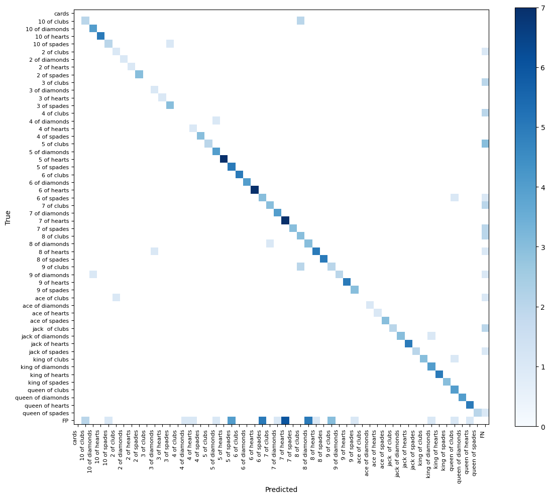
print(f"map75: {mean_average_precision.map75:.2f}")A confusion matrix is a table summarizing the performance of a classification algorithm, showing the number of correct and incorrect predictions for each class. In the context of object detection, it reveals the distribution of true positives, false positives, true negatives, and false negatives. The vast majority of detections are on the diagonal of our confusion matrix, meaning both the bounding box and the class of our detection are correct. The only weak point of our model is a significant number of false negatives, which are objects that are present in the ground truth but not detected by the model. This is most likely due to class imbalance in the dataset.
Conclusion
RT-DETR is one of the top object detectors. Its unique combination of state-of-the-art speed and accuracy, along with a fully open-source license, makes it an excellent choice, especially for open-source projects.
With its recent integration into the Transformers library, fine-tuning RT-DETR on custom datasets has become more accessible than ever before, opening up new possibilities for object detection applications.
Explore the accompanying notebook for a more hands-on experience and to experiment with different datasets and configurations.
Cite this Post
Use the following entry to cite this post in your research:
Piotr Skalski. (Jul 11, 2024). How to Train RT-DETR on a Custom Dataset with Transformers. Roboflow Blog: https://blog.roboflow.com/train-rt-detr-custom-dataset-transformers/