The tides of open source machine learning technology advance with the integration of YOLOS (You Only Look at One Sequence) into the Hugging Face Transformers library. If you're new to YOLOS and interested in the architecture, we have a specific YOLOS breakdown post.
In this post, we showcase the power of combining a suite of best-in-class machine learning tools - Hugging Face Transformers, Roboflow, Weights and Biases, and AWS Sagemaker Serverless - to create a YOLOS object detection labeling, training, and deployment pipeline.
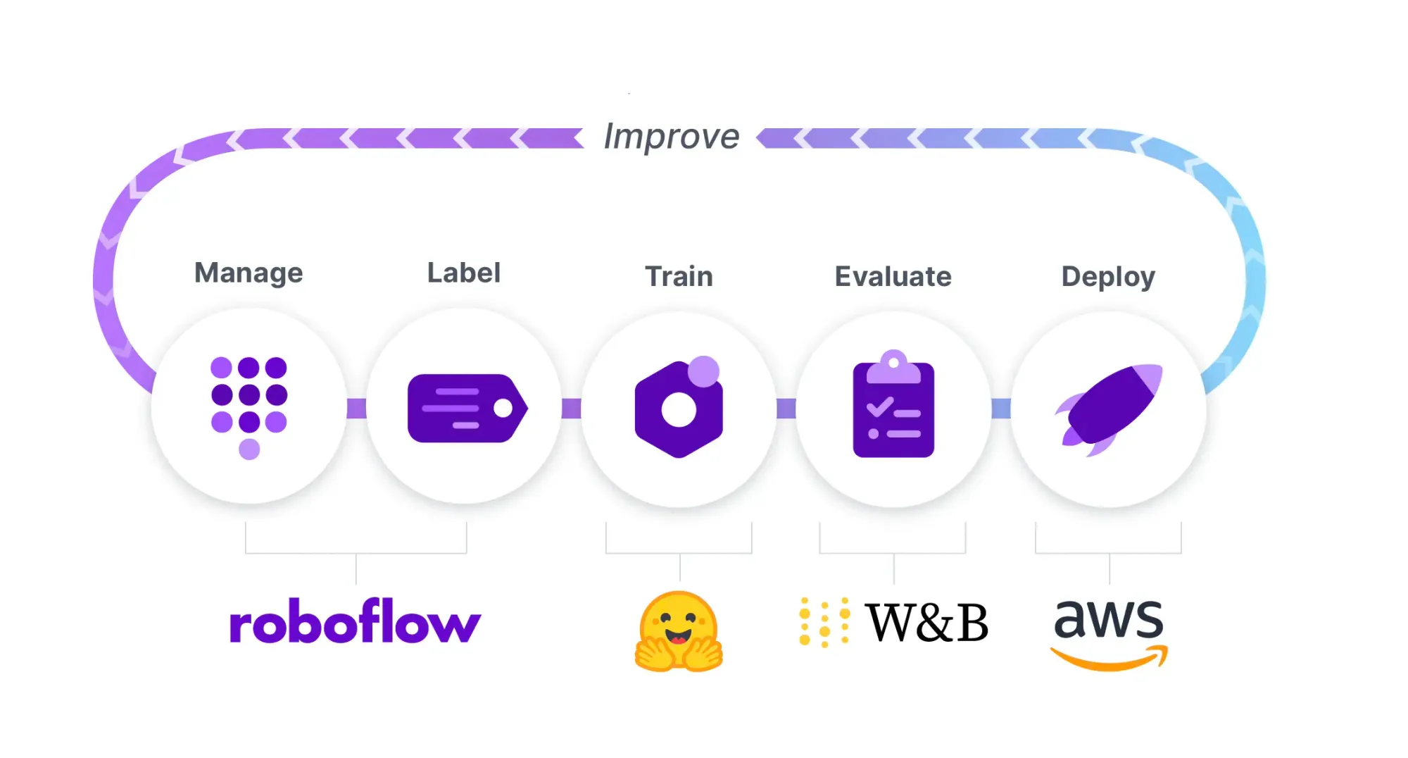
In order to train and deploy YOLOS, we will perform the following steps in an example how to train YOLOS notebook:
- Install YOLOS Environment
- Gather and Label Our Dataset in Roboflow
- Download Our Dataset and Prepare Data For Training
- Configure Our YOLOS Model from Hugging Face Transformers
- Run Custom YOLOS Training in PyTorch Lightning
- Visualize YOLOS Training in Weights and Biases
- Evaluate Custom YOLOS Model
- Visualize Test Inference
- Deploy YOLOS Model to AWS Sagemaker Serverless
- Sample images for Active Learning with Roboflow to improve our model
We recommend having the notebook up alongside this blog post.
Why We're Excited About YOLOS
In the world of computer vision modeling, the latest and greatest models have been formulated from Transformer architectures, which were originally built for NLP tasks, and have since taken the AI world by storm.
The first of these was the Vision Transformer (ViT) which set new records on the task of image classification.
It was only a matter of time before researchers began experimenting with adapting the vision transformer to other tasks in computer vision, and along came YOLOS to apply ViT to object detection.
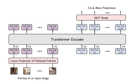
YOLOS looks at patches of an image to form "patch tokens", which are used in place of the traditional wordpiece tokens in NLP. There are 100 detection tokens appended on the right, which are learnable embeddings that each look for a particular object in an image.
Compared to other CNN-based YOLO models, YOLOS benefits from the rising tides of Transformers in computer vision, as well as inferring without the need for NMS, a tedious post-processing step that makes the deployment of other YOLO models difficult and slow.
Let's dive into training YOLOS.
Install YOLOS Environment
We start by building the dependencies necessary for training YOLOS by installing some awesome machine learning packages pytorch-lightning ⚡️, transformers 🤗, wandb, and roboflow. We will import the YOLOS model architecture implementation from transformers and we will use pytorch-lightning for our training routine, and visualize in wandb.
!pip install -q transformers
!pip install -q pytorch-lightning
!pip install -q wandb
!pip install -q roboflowFor deployment, we will be using AWS Sagemaker Serverless:
!pip install sagemaker --upgrade -q
!curl "https://awscli.amazonaws.com/awscli-exe-linux-x86_64.zip" -o "awscliv2.zip"
!unzip awscliv2.zip
!sudo ./aws/install
After you have these installs, you need to login to wandb, and if you're deploying, provide your AWS credentials.
Assembling Our Dataset
It's all about the data! Your model is only as good as the data you feed into it for training.
In order to train our custom model, we need to assemble a dataset of representative images with bounding box annotations around the objects that we want to detect. It is absolutely essential to gather your own, real world images, that closely reflect the ones your deployed application will see in the wild if you want to build a performant model.
Therefore, for this tutorial we recommend that you:
- Upload raw images and annotate them in Roboflow with Roboflow Annotate
For the purposes of the tutorial, you can also
- Convert an existing dataset to COCO format. Roboflow supports over 30 formats object detection formats for conversion
- Browse and download open source object detections projects to start from on Roboflow Universe
- Use the same Blood Cell Detection dataset we use in this tutorial
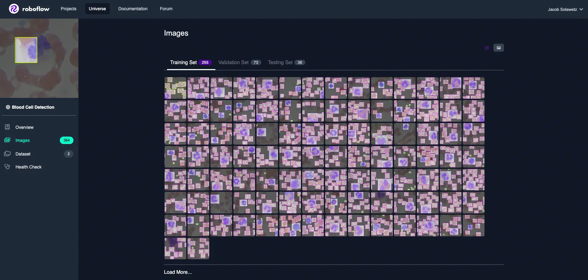
After you hit Export on your dataset version in Roboflow, select the COCO format and you will receive a Python snippet to download your dataset into your Colab notebook. It should look something like this:
rf = Roboflow(api_key="YOUR_KEY_HERE")
project = rf.workspace("YOUR_WORKSPACE").project("YOUR_PROJECT")
dataset = project.version(YOUR_VERSION).download("coco")
Then we register our dataset with the torchvision implementation of the COCO dataset format, and build the dataloader that we will later use in training.
#Register dataset as torchvision CocoDetection
import torchvision
import os

class CocoDetection(torchvision.datasets.CocoDetection):
    def __init__(self, img_folder, feature_extractor, train=True):
        ann_file = os.path.join(img_folder, "_annotations.coco.json")
        super(CocoDetection, self).__init__(img_folder, ann_file)
        self.feature_extractor = feature_extractor

    def __getitem__(self, idx):
        # read in PIL image and target in COCO format
        img, target = super(CocoDetection, self).__getitem__(idx)

        # preprocess image and target (converting target to DETR format, resizing + normalization of both image and target)
        image_id = self.ids[idx]
        target = {'image_id': image_id, 'annotations': target}
        encoding = self.feature_extractor(images=img, annotations=target, return_tensors="pt")
        pixel_values = encoding["pixel_values"].squeeze() # remove batch dimension
        target = encoding["labels"][0] # remove batch dimension

        return pixel_values, target

from transformers import AutoFeatureExtractor

feature_extractor = AutoFeatureExtractor.from_pretrained("hustvl/yolos-small", size=512, max_size=864)

train_dataset = CocoDetection(img_folder=(dataset.location + '/train'), feature_extractor=feature_extractor)
val_dataset = CocoDetection(img_folder=(dataset.location + '/valid'), feature_extractor=feature_extractor, train=False)

print("Number of training examples:", len(train_dataset))
print("Number of validation examples:", len(val_dataset))
We double check that our data loaded correctly by checking the length of our training and validation set objects.
Number of training examples: 255
Number of validation examples: 73
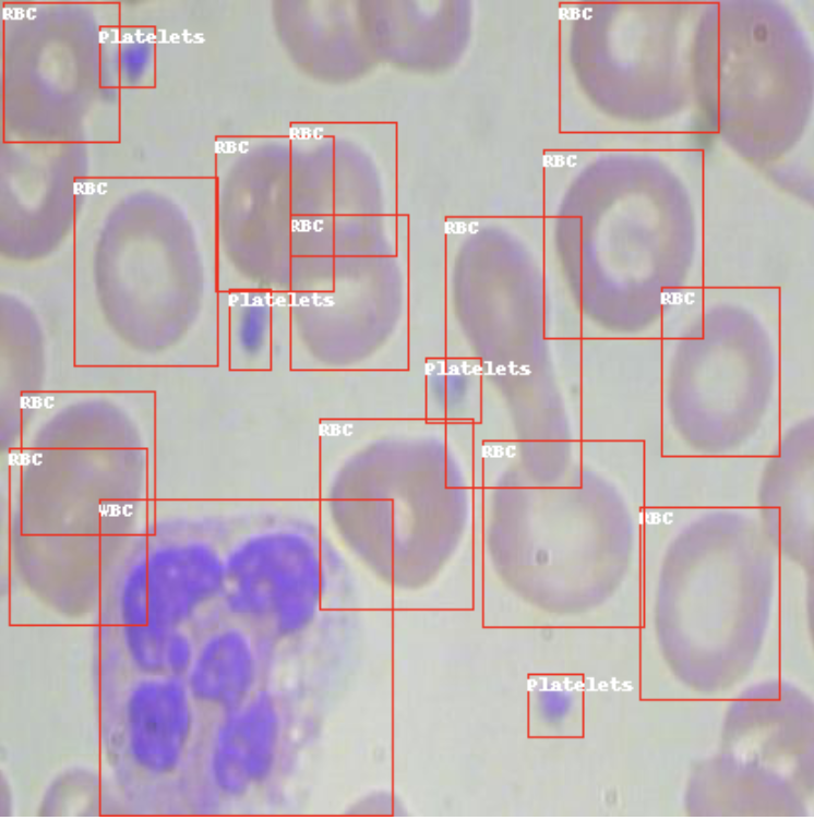
And to be doubly sure that the annotations loaded correctly, we plot them on a sample image from the training set.
Setting Up YOLOS Training Configuration
Next we set up the training configuration, importing an immense amount of functionality from transformers and pytorch-lightning.
We start by importing the entirety of the model definition:
self.model = AutoModelForObjectDetection.from_pretrained("hustvl/yolos-small")Note - here we chose the yolos-small model which is 117 mb in size. You can also choose the yolos-tiny model, 24 mb for faster training, inference, but lessor accuracy. If training and inference time are not a concern, you can train the yolos-base model, 488 mb for higher accuracy.
Then, we wrap our model in a pl.LightningModule training loop.
Finally we initialize our model:
model = YoloS(lr=2.5e-5, weight_decay=1e-4)And that's it! We are ready to train.
Run Custom YOLOS Training
Next, we kick off training:
from pytorch_lightning import Trainer

trainer = Trainer(gpus=1, max_epochs=10, gradient_clip_val=0.1, accumulate_grad_batches=8, logger=wandb_logger)
trainer.fit(model)Visualize YOLOS Training and Track Experiments
While our model is training, we can log in to our Weights and Biases dashboard to visualize training. As your model trains, it will cycle through the example images and annotations that you have provided it and tune its weights to more accurately model the task you have given it.
In Weights and Biases, you get to watch the validation loss of your model descend.
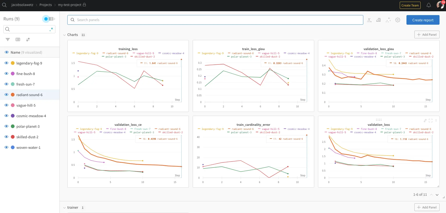
You can also track your experiments side by side, to see how your dataset or your modeling technique is improving over previous iterations.
Evaluate Custom YOLOS Model
After we have trained our YOLOS model, we want to evaluate it to see if we have trained it well, or else, we have more work to do on our dataset.
We first use the COCO evaluator to print out detailed evaluation across mean average precision thresholds.
IoU metric: bbox
 Average Precision  (AP) @[ IoU=0.50:0.95 | area=   all | maxDets=100 ] = 0.036
 Average Precision  (AP) @[ IoU=0.50      | area=   all | maxDets=100 ] = 0.058
 Average Precision  (AP) @[ IoU=0.75      | area=   all | maxDets=100 ] = 0.044
 Average Precision  (AP) @[ IoU=0.50:0.95 | area= small | maxDets=100 ] = 0.003
 Average Precision  (AP) @[ IoU=0.50:0.95 | area=medium | maxDets=100 ] = 0.010
 Average Precision  (AP) @[ IoU=0.50:0.95 | area= large | maxDets=100 ] = 0.423
 Average Recall     (AR) @[ IoU=0.50:0.95 | area=   all | maxDets=  1 ] = 0.030
 Average Recall     (AR) @[ IoU=0.50:0.95 | area=   all | maxDets= 10 ] = 0.074
 Average Recall     (AR) @[ IoU=0.50:0.95 | area=   all | maxDets=100 ] = 0.120
 Average Recall     (AR) @[ IoU=0.50:0.95 | area= small | maxDets=100 ] = 0.019
 Average Recall     (AR) @[ IoU=0.50:0.95 | area=medium | maxDets=100 ] = 0.177
 Average Recall     (AR) @[ IoU=0.50:0.95 | area= large | maxDets=100 ] = 0.750
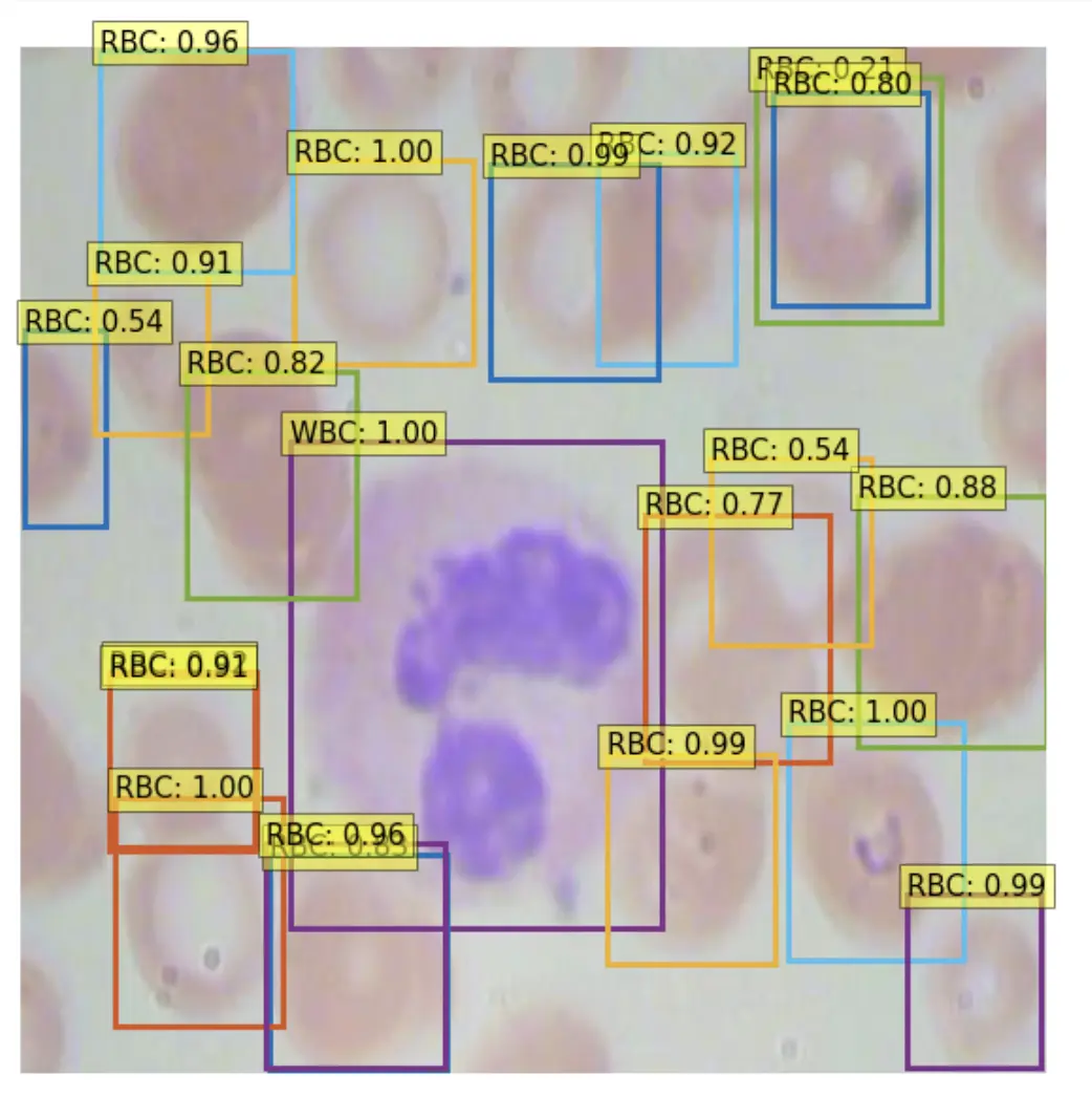
Then we can perform test inference, to verify that our model is making acceptable inference on a test image.
Deploy YOLOS Model to AWS Sagemaker Serverless
Once we have a model that we are satisfied with, we need to deploy it for it to be useful for feeding predictions to a production application. In this part of the notebook, we showcase using AWS Sagemaker Serverless for cloud deployment.
other deployment options
Sagemaker Serverless scales our model for us, taking care of all of the complicated cloud architecting we would normally need to do to scale compute instances that are serving our model up and down.
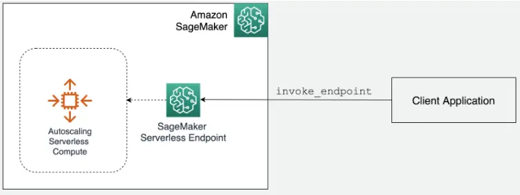
To deploy to Sagemaker, we package our model artifacts along with preprocessing instructions into a deployment folder:
/content/deploy
code/
code/inference.py
code/requirements.txt
config.json
model.tar.gz
preprocessor_config.json
pytorch_model.bin
Then, we upload these specifications of our model to S3 and then to Sagemaker using the sagemaker SDK.
from sagemaker.huggingface.model import HuggingFaceModel
from sagemaker.serverless import ServerlessInferenceConfig
from sagemaker.serializers import DataSerializer

huggingface_model_sls = HuggingFaceModel(
   model_data=s3_location,  # path to your trained sagemaker model in S3
   #env=hub,
   role=role, # iam role with permissions to create an Endpoint
   transformers_version="4.17", # transformers version used
   pytorch_version="1.10", # pytorch version used
   py_version="py38", # python version of the DLC
)

serverless_config = ServerlessInferenceConfig(
    memory_size_in_mb=4096, max_concurrency=10,
)

# create a serializer for the data
image_serializer = DataSerializer(content_type='image/x-image') # using x-image to support multiple image format

predictor_sls = huggingface_model_sls.deploy(
    serverless_inference_config=serverless_config,
    serializer=image_serializer, # serializer for our audio data.
)This will take a while as our model is registered with AWS and loaded into a container that will serve our inference.
Once that completes, our model is read to be invoked for inference!
image_path = "YOUR_IMAGE_PATH"

res = predictor_sls.predict(data=image_path)
You can then log into the AWS console in Sagemaker to view a dashboard containing details about our model's deployment and log streams.
YOLOS Active Learning
It is important to note that our model will not always perform perfectly. In the wild, there will be all kinds of edge cases that break our model. This is because, the model we have made is only as good as the data we have given trained it on.
In order to improve our model when an edge case is found, we need add the new data to our dataset, and complete the loop again - iterating on our approach. We can upload new data to Roboflow using the same project object that we downloaded our dataset with so that the more real world scenarios our model encounters, the more it can learn, and the better it can get.
project.upload(image_path)You may implement intelligent active learning rules - for example, you may want to upload when your model finds no objects with confidence greater than 40%
min_box_conf = float("inf")
for box in res:
    if box["score"] < min_box_conf:
        min_box_conf = box["score"]
if min_box_conf < 0.4:
    project.upload(image_path)
Conclusion
Congratulations! Now you know how to train YOLOS to detect objects specific to your custom task.
In this blog post, we showcased some of the best of what machine learning technology has to offer by combining a powerful suite of tools for the task:
- Roboflow for dataset management and active learning
- Hugging Face Transformers for modeling
- Weights and Biases for experiment tracking
- AWS Sagemaker Serverless for deployment
We hope you enjoyed - happy training! And happy inference!
And in case you missed it above: here is the link to the How to Train YOLOS Notebook. For more information on YOLOS, we have a post explaining the architecture in more detail.
Cite this Post
Use the following entry to cite this post in your research:
Jacob Solawetz, Mark McQuade. (Jun 15, 2022). Train and Deploy YOLOS Transformer On a Custom Dataset. Roboflow Blog: https://blog.roboflow.com/train-yolos-transformer-custom-dataset/
