What Is Neural Architecture Search?

Designing a neural network is a challenging task, requiring mixing and matching layers, activation functions, and connection patterns until a winning combination is achieved. And today’s deep learning models are often massive image models with many layers, or language models with billions of parameters, making manually designing the perfect neural network architecture much more difficult.

Neural Architecture Search (NAS) has emerged as an answer to this challenge. NAS techniques treat neural‑network design as a machine‑learning problem. Rather than manually building a model architecture, an algorithm searches a space of candidate architecture, and automatically discovers a configuration that meets user‑defined objectives.

This paradigm belongs to the broader field of Automated Machine Learning (AutoML) and is closely related to hyper‑parameter optimization and meta‑learning.

In recent years, NAS has produced models such as NASNet, EfficientNet, AlphaNet and YOLO-NAS which often perform as well as or even better than models designed by humans, while using fewer resources. Modern NAS methods have also improved to use less energy than early versions.

In this blog post, you’ll learn the following:

• What is NAS?
• The main components of NAS systems.
• How NAS works.
• The types of search spaces and strategies in NAS.
• Why NAS is useful.

So, let’s get started.

What Is Neural Architecture Search?

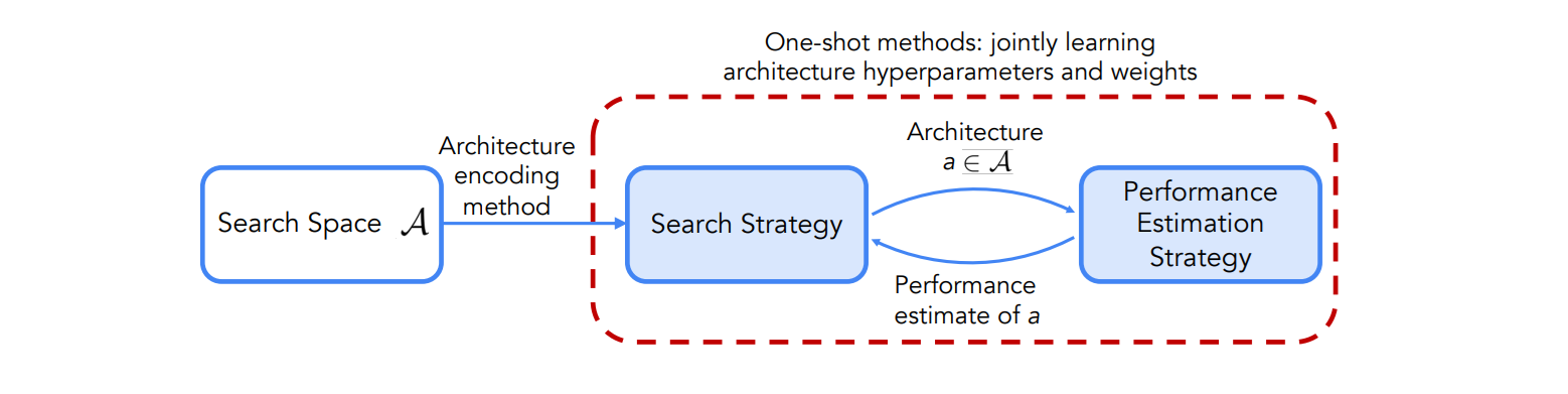
Neural architecture search is a technique for automating the design of artificial neural networks. Given a specific task (e.g., image classification, object detection, language modeling or image segmentation), a NAS algorithm searches over a pre‑defined space of possible neural‑network topologies to find an architecture that optimizes a performance metric such as accuracy, latency, or model size. The key components of NAS are as follows:

Search Space

The search space specifies the kinds of architectures that the algorithm may consider. This includes allowable operations (such as convolution, pooling, attention layers, fully connected layers, and activation functions, etc.), how these operations can be combined, and hyper‑parameters such as kernel size or number of channels. The search space may be global covering complete networks, or modular, where the algorithm learns reusable cells or blocks that can be stacked to build deeper models.

Search Strategy

The search strategy (or controller) is an algorithm that proposes candidate architectures from the search space and updates its proposals based on feedback. Common strategies include random sampling, reinforcement learning systems that build architectures step by step and adjust based on test results, and evolutionary algorithms that improve a group of architectures through mutation and selection. Other methods include Bayesian optimization, step-by-step model-based search (also called progressive search), and gradient-based approaches that optimize architecture settings alongside network weights in a continuous search space.

Performance Estimation Strategy

Evaluating each candidate architecture by fully training it can be excessively expensive. Performance estimation strategies speed up evaluation using proxy tasks (e.g., training on reduced datasets or fewer epochs), replacement or substitute models that predict a model’s performance from its structure, or weight‑sharing/one‑shot approaches that train a large supernetwork containing all possible operations and then evaluate different sub‑architectures using shared weights.

NAS benchmarks have been introduced to provide datasets and precomputed results that allow quick performance estimation and reduce the carbon footprint of NAS.

These three components: search space, search strategy and performance estimation, are the building blocks of any NAS framework. Next, we examine how NAS algorithms actually work by stepping through a typical NAS process, and surveying the most common search strategies.

How Does NAS Work?

A general NAS workflow can be summarized in following steps:

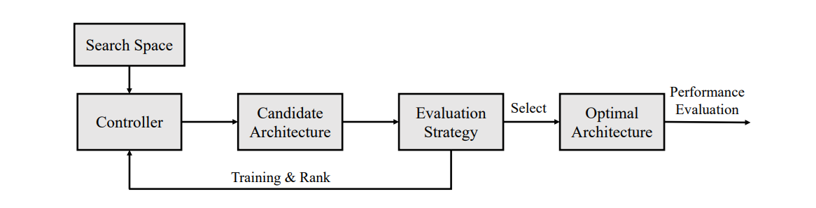
Step #1: Define the search space

In this step a set of operations (e.g., convolution, pooling, recurrent layers) and possible connections among them are decided. These operations form the building blocks for candidate architectures. The search space can be extremely large if it considers all possible layer combinations, so many NAS methods restrict the search to specific templates (such as cell‑based or hierarchical structures).

Step #2: Generate candidate architectures

A controller (the search strategy) proposes architectures from the search space. The controller might randomly sample, follow a policy learned by reinforcement learning, mutate existing architectures in an evolutionary loop, or adjust architecture parameters using gradients.

Step #3: Evaluate candidates

Each proposed architecture is partially or fully trained on a dataset. Its performance is then recorded on a validation set. To reduce cost, evaluation may involve training only a few epochs or using substitute models to estimate performance. In one‑shot approaches the architecture’s weights are inherited from a supernetwork rather than trained from scratch.

Step #4: Update the search strategy

The controller uses feedback from evaluated architectures to refine its search. In reinforcement learning methods, the controller updates its policy to pick better architectures. In evolutionary strategies, low‑performing candidates are replaced by modified versions of high‑performing candidates. In gradient‑based NAS, the architecture parameters are adjusted via back‑propagation over a continuous relaxation of the search space.

Step #5: Iterate and finalize

Steps 2 to 4 are repeated until the search meets a termination condition (e.g., a maximum number of evaluations or convergence of validation performance). Finally, the best architecture is fully trained on the training dataset and evaluated on the test set to report its performance.

Types of Search Space in NAS

The search space defines the set of all possible architectures the algorithm can explore. It acts as the “design playground,” specifying what building blocks (such as layers, blocks, or cells) are available and how they can be connected. The choice of search space heavily influences both the expressiveness of the architectures that can be discovered and the efficiency of the search process. Let’s discuss common search space types.

Macro Search Spaces

The macro search space defines the entire neural network architecture in a single stage rather than focusing on smaller repeated components. It has two variants:

• In one variant, the architecture is modeled as a directed acyclic graph (DAG) where each node represents an operation (such as convolution, pooling, or fully connected layers) and the search includes both the choice of operations and the network topology. For example, the NASBOT CNN search space allows combinations of various convolution and pooling layers with depths up to 25.
• In another variant, the topology and operations remain fixed, but macro-level hyperparameters such as network depth, width, and spatial resolution downsampling points are optimized, such as scaling strategy in EfficientNet.

While macro search spaces provide high expressiveness and the potential to discover entirely novel architectures, their vast design space makes them computationally expensive to explore.

Chain-Structured Search Spaces

The chain-structured search space defines architecture as a simple sequential stack of layers, where each layer directly feeds into the next. These spaces often build on strong manually designed backbones such as ResNet or MobileNet and then allow variation in certain components.

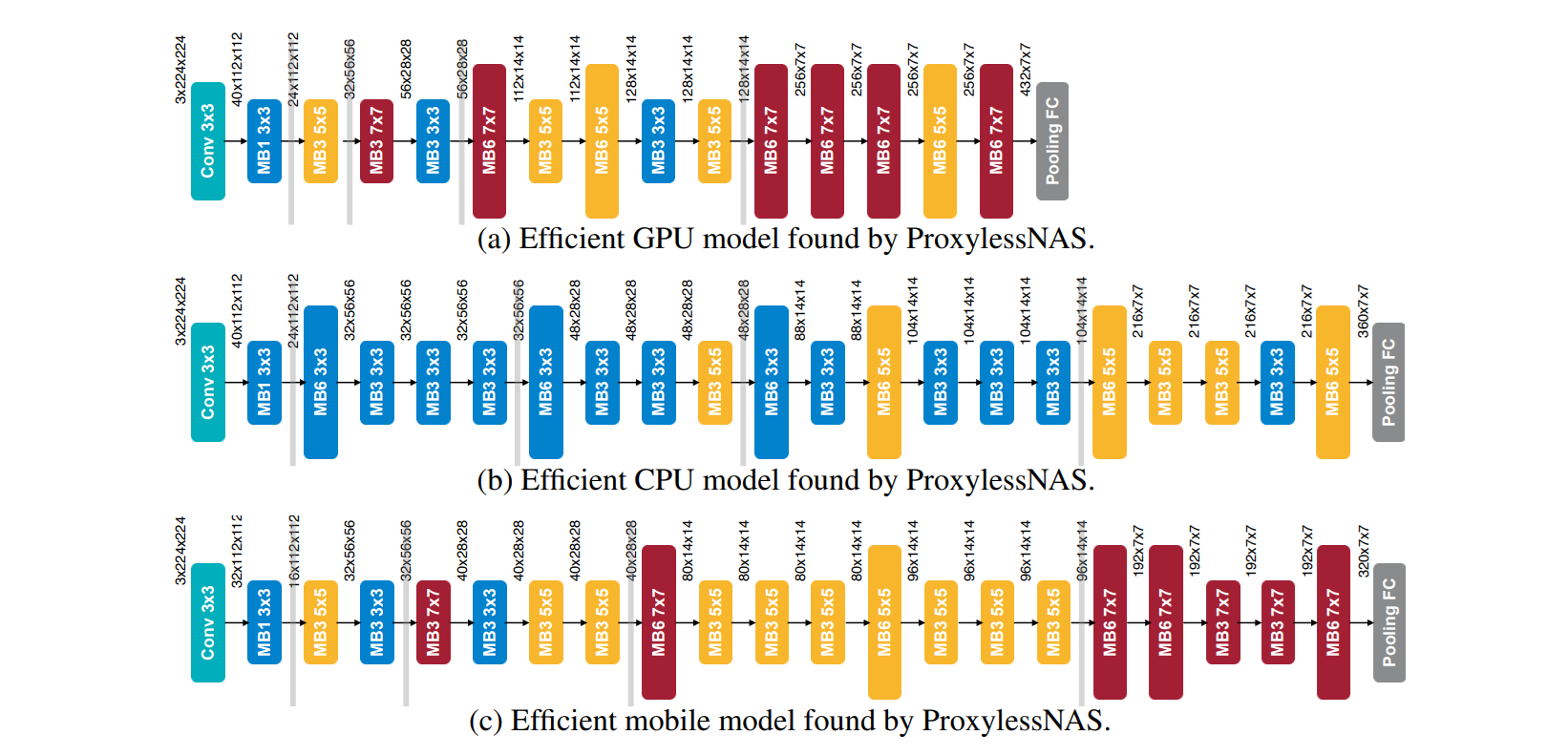
For example, ProxylessNAS starts from MobileNetV2 and searches over kernel sizes and expansion ratios in inverted bottleneck residual layers, while XD-operations and DASH explore kernel sizes, dilations, or generalized convolutions derived from LeNet, ResNet, or WideResNet.

Chain-structured designs are also common in transformer-based NAS. Lightweight Transformer Search (LTS) searches GPT-style models by varying layer count, model width, embedding dimensions, feedforward network size, and attention heads. NAS-BERT and MAGIC apply similar ideas to the BERT architecture with multiple attention, feedforward layers, and convolutions with different kernel sizes.

This design is easy to implement, computationally efficient to search, and can quickly yield competitive models. But the restricted linear topology limits the diversity of architectures, and reduces the likelihood of discovering highly novel designs.

Cell-Based Search Space

Cell-based search space focuses on designing small, repeatable building blocks (cells) instead of searching the entire network from scratch. This idea comes from human-designed CNNs like ResNet, where repeating units such as residual blocks are used throughout the model. In this setup, the micro-structure (the cell’s internal design) is searched, while the macro-structure (how cells are arranged in the full network) is fixed.

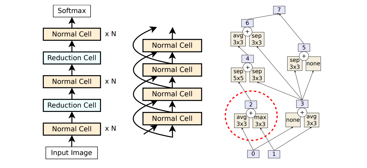
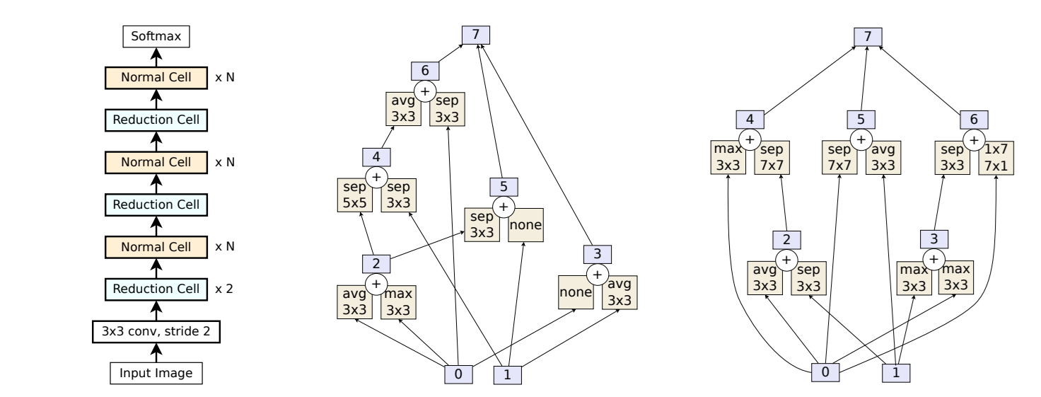
The first well-known example, NASNet, uses two cell types:

• Normal cell keeps the same spatial resolution.
• Reduction cell halves the spatial resolution by using stride-2 operations.

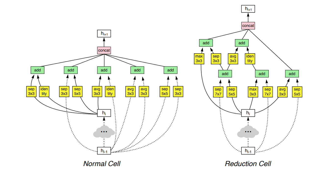
Each cell is a DAG with nodes representing operations (e.g., convolutions, pooling) and combination steps (addition or concatenation). By stacking normal and reduction cells, NASNet produces the final architecture.

Other popular cell-based spaces include NAS-Bench-101, which defines 7-node cells with 3 operation choices per node (423,624 possible architectures), and DARTS, which differs by placing operations on the edges of the graph rather than the nodes and allow gradient-based search and yielding 10¹⁸ possible architectures.

Cell-based designs are also applied beyond computer vision tasks. For example, NAS-Bench-ASR searches convolutional cells for speech recognition, and LSTM-based cell search spaces exist for language modeling.

The main strength of cell-based search is efficiency and transferability. Optimal cells found on small datasets like CIFAR-10 can be scaled up for larger datasets like ImageNet. However, limitations include low performance variance among architectures (making advanced search strategies yield small gains), ad-hoc design constraints (like fixed cell node counts), and reduced expressiveness compared to macro-level search.

Hierarchical Search Space

The hierarchical search space designs architectures at multiple levels rather than searching only one flat level (like in the cell or macro level). In this approach, higher-level motifs are built from lower-level motifs, and each level is typically represented as a DAG composed of components from the level below.

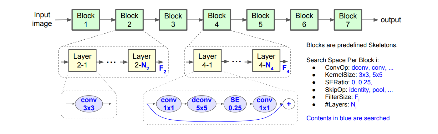
A simple example is a two-level hierarchy, where the lower level defines the micro-structure (such as cells or layer blocks) and the upper level controls macro-level hyperparameters like the number of cells per stage, downsampling points, or block types.

For example, MnasNet uses MobileNetV2 blocks at the lower level and searches macro parameters like depth, width, and resolution at the higher level. Similar two-level setups have been applied in semantic segmentation, image denoising, stereo matching, and vision transformers, combining local convolutions and global self-attention layers.

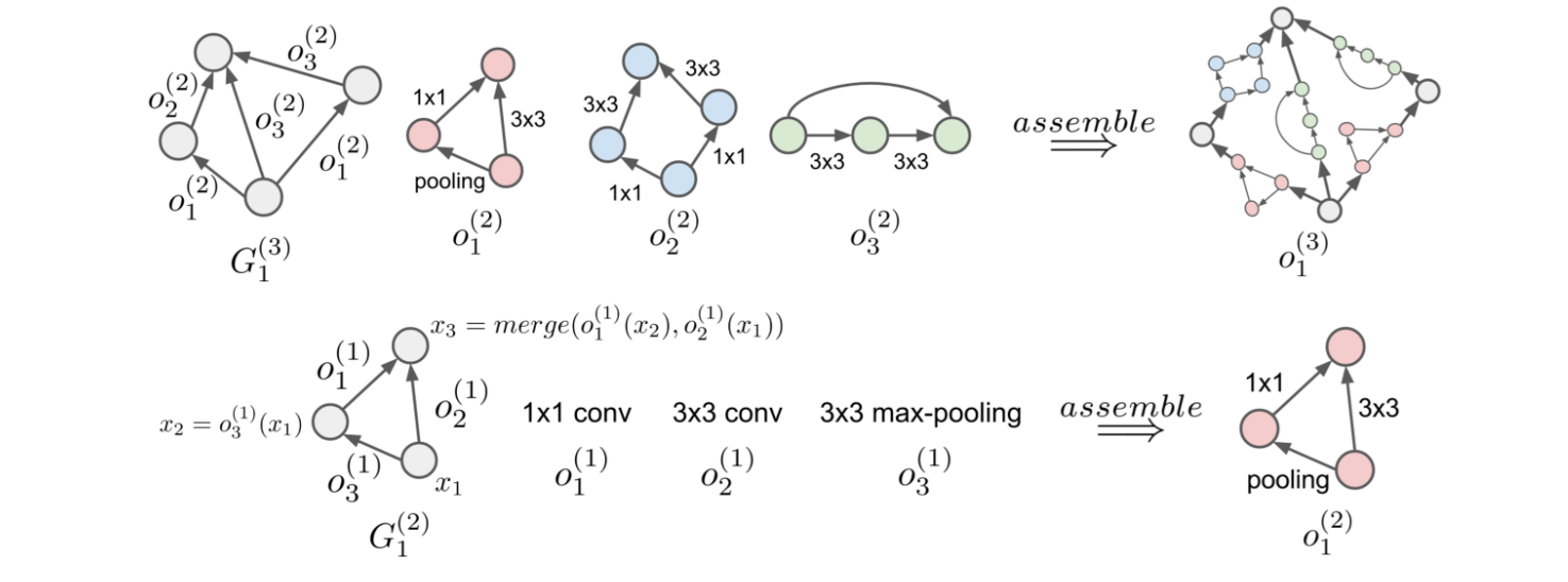
More complex designs extend this to three or more levels where:

• Level 1 defines primitive operations i.e. smallest building blocks such as a 3x3 convolution, max pooling, or a ReLU activation. For example, A 3×3 Conv layer from ResNet.
• Level 2 defines motifs, a small structures made by combining multiple primitives into a reusable unit. For example, a ResNet residual block combining convolution, batch normalization, and skip connections.
• Level 3 defines the final architecture i.e. the complete network formed by connecting multiple motifs in sequence or stages. For example, ResNet-50, which stacks residual blocks into four main stages to form the full model.

There are researches that extend beyond three levels, enabling recursive or variable-depth hierarchies for even more complex designs.

The hierarchical search space is highly expressive, and able to represent a much wider variety of architectures. It can reduce search complexity by reusing smaller motifs to build larger structures. However, it is more complex to implement, and requires careful design to make the search efficient.

Search Strategies in NAS

The search strategy is the method NAS uses to explore the search space and find high-performing architectures. Different strategies balance exploration (trying new designs) and exploitation (refining promising ones) in different ways.

Reinforcement Learning (RL)

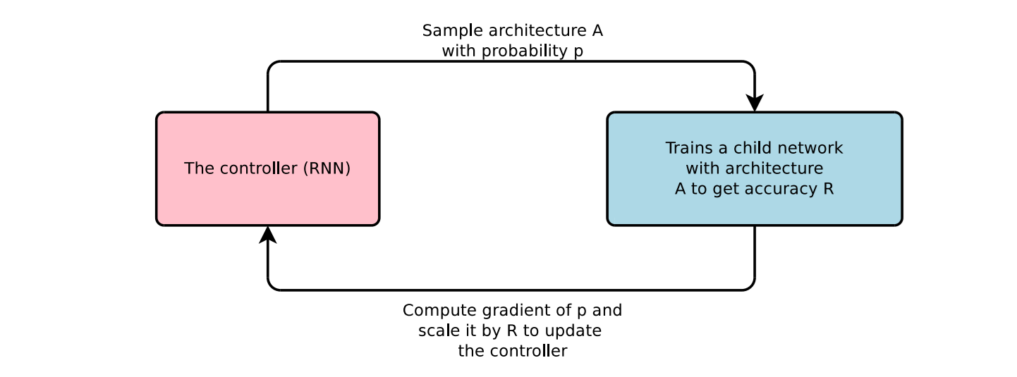
In the reinforcement learning based NAS search technique, an agent (often implemented as a RNN controller) generates architectures step-by-step by making sequential decisions about layers, operations, and connections. After an architecture is generated, it is trained and evaluated on a target task, and the resulting performance (e.g., validation accuracy) is used as a reward signal. Over many iterations, the controller learns to produce better architectures by maximizing these rewards. This approach treats architecture search as a sequential decision-making problem, allowing the system to explore vast and complex design spaces.

A famous example is NASNet which used RL to discover high-performing convolutional cell structures that could be transferred to larger datasets like ImageNet. Another example is ENAS, which improved efficiency by using parameter sharing so that multiple architectures could reuse weights. This reduces the search cost from many GPU days to just a few.

Evolutionary Algorithms (EA)

Evolutionary algorithms mimic the process of natural selection to discover optimal architectures. They maintain a collection of candidate architectures (population), evaluate their performance (fitness), and select the best-performing models by altering layers, kernel sizes, or connections (mutation) and combining parts of two architectures (crossover). Over iterations, the model evolves toward better design.

One well-known approach, AmoebaNet-A is an image classifier, outperforming many manually designed architectures. Another early milestone was Large-Scale Evolution of Image Classifiers, which demonstrated that pure evolutionary methods could compete with human-designed models when given sufficient computational resources. However, powerful EA can be expensive since evaluating each generation often requires training many architectures from scratch.

Gradient-Based / Differentiable Search

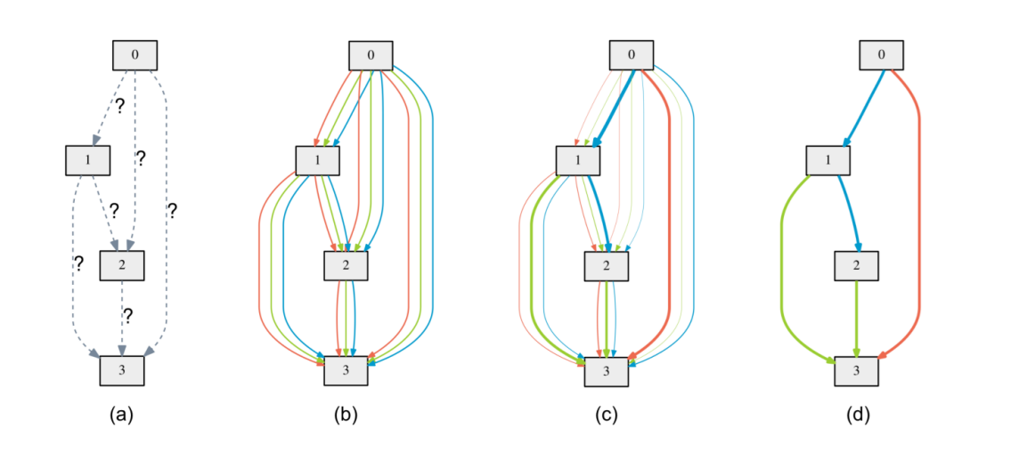
Gradient-based NAS transforms the discrete architecture search problem into a continuous optimization problem. Instead of choosing one operation for each connection, it assigns continuous weights to all possible operations (via softmax relaxation). Both the model’s weights and these architecture parameters are optimized together using gradient descent. At the end, the highest-weighted operations are selected to form the final architecture.

The DARTS method initiated this approach by enabling fast search without training each candidate from scratch. Later improvements like ProxylessNAS adapted this method to run directly on target hardware while keeping memory usage low. Gradient-based NAS offers high speed improvements compared to RL or EA but can sometimes due to relaxation, the search can settle on designs that are not the best.

Bayesian Optimization (BO)

Bayesian optimization is a sample-efficient NAS method that builds a probabilistic model (often a Gaussian process) to approximate the relationship between architecture configurations and their performance. Using this model, it selects the next architecture to try via an acquisition function, which balances exploring new regions of the search space and exploiting known promising areas.

For example, NASBOT used Bayesian optimization combined with optimal transport metrics to guide the search in complex CNN architecture spaces. BO is particularly useful when training each candidate is computationally expensive, because it can find good architectures with fewer evaluations. However, it struggles in extremely large or high-dimensional search spaces.

Random Search

Random search is the simplest NAS strategy. It selects architectures completely at random from the search space, trains them, and records performance. While this brute-force approach lacks intelligent guidance, research has shown that with a well-designed search space, random search can be surprisingly competitive. Especially when paired with weight sharing to reduce evaluation costs.

Liam Li and Ameet Talwalkar showed that a carefully controlled random search can perform well in some cases. But without learning-based guidance, random search usually needs many more tries to find good models. So it becomes costly in very large search spaces.

One-Shot NAS (Supernet-Based Search)

One-shot NAS trains a supernet, a single large network that contains all possible sub-architectures in the search space as paths or subgraphs. Candidate architectures are evaluated by sampling subnets from the supernet and using the already-trained shared weights which avoid full retraining. This “train once, evaluate many” strategy reduces search time.

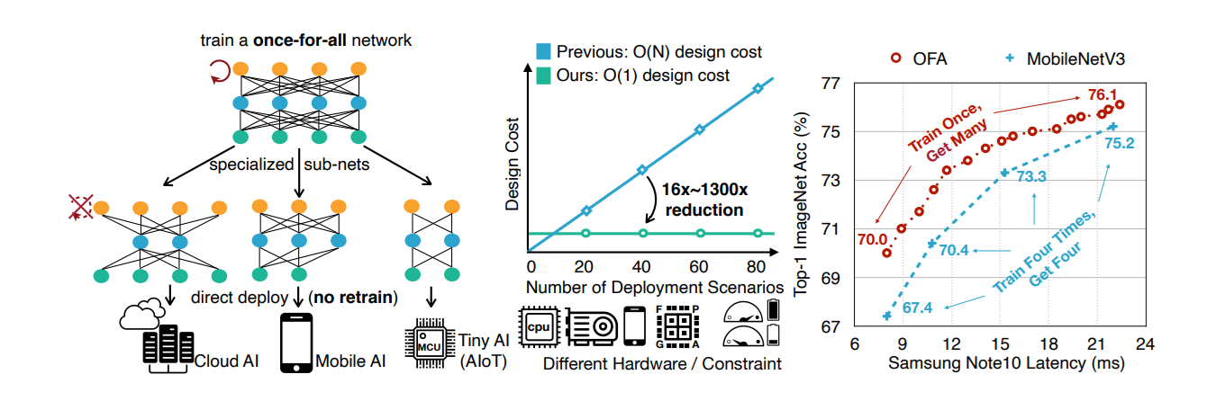
The Once-for-All Network  is a prime example, where the supernet is trained to support many configurations that can be specialized for different devices or constraints (e.g., latency, power consumption). One-shot NAS provides speed and flexibility but can introduce bias, as shared weights may not perfectly reflect the performance of individually trained architectures.

Why Use Neural Architecture Search?

NAS offers a smarter, automated way to design deep learning models, removing much of the guesswork and manual trial-and-error involved in traditional architecture creation. By systematically exploring a wide range of design possibilities, NAS can find architectures that are not only accurate, but also efficient and tailored to specific hardware needs.

From discovering completely new structures that outperform human-designed models, to creating lightweight, low-latency networks for mobile and edge devices, NAS enables faster innovation, better performance, and models that can generalize across tasks all while supporting multi-objective goals such as reduced memory footprint, energy efficiency, and even lower carbon emissions.

Automation and Accessibility

One of the primary benefits of NAS is reducing the need for manual trial‑and‑error. Traditional neural‑network design often requires significant domain knowledge and time‑consuming experimentation. NAS automates this process and allows even non‑experts to obtain high‑performing models.

Discovery of Novel Architectures

NAS can uncover network designs that humans might not have considered. For example, NASNet’s cell‑based architecture achieved higher accuracy on CIFAR‑10 and ImageNet than manually designed models, while using fewer floating‑point operations. EfficientNet, a family of convolutional networks discovered using a combination of NAS and compound scaling, provide state‑of‑the‑art accuracy while being far more parameter‑efficient than prior models.

Efficiency and Hardware Awareness

NAS enables models to be customized to specific hardware constraints. Multi‑objective NAS frameworks optimize not only accuracy, but also inference latency, energy consumption, and memory usage. Techniques like DPP‑Net explicitly incorporate device characteristics (e.g., memory capacity) into the search process, while ProxylessNAS searches directly on the target hardware by pruning computational paths.

These hardware‑aware NAS can generate lightweight models suitable for mobile devices or real‑time applications, which is increasingly important for deploying AI at the edge.

Faster Development and Iteration

NAS automates network design to shorten the development cycle. NAS automatically explores a wide range of architectures and identifies the best ones based on predefined criteria. Weight‑sharing and differentiable NAS reduce search times to a few days or even hours. This accelerated iteration helps to explore new ideas more rapidly and deliver models to production faster.

Generalization and Transferability

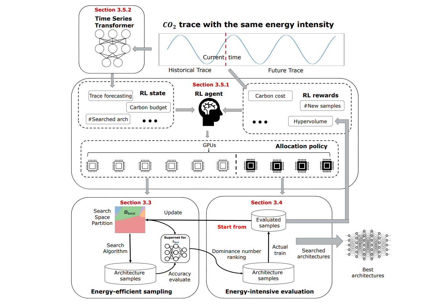
Architecture modules discovered by NAS often generalize across tasks and datasets. For example, the cells learned by NASNet on CIFAR‑10 were successfully transferred to ImageNet and improved object‑detection performance when integrated into the Faster‑RCNN framework. Transferability reduces the need to perform a costly search for every new task, as reusable building blocks can be fine‑tuned or combined for different applications.

Multi‑Objective and Sustainable AI

Maximizing accuracy of a model alone is not sufficient. Many real‑world applications must consider trade‑offs such as memory footprint, latency, energy consumption, etc. Multi‑objective NAS frameworks like LEMONADE optimize multiple objectives such as accuracy, memory requirements, and latency. Also, carbon‑efficient NAS search frameworks such as CE‑NAS reduce compute requirements and address carbon footprint.

Conclusion

Neural architecture search has transformed the way we design neural networks. By treating architecture design as a learning problem and automating the search over network topologies, NAS allows discovery of high‑performing, efficient models. Core components of NAS (search spaces, search strategies, and performance estimation) define the framework through which NAS operates.

Search strategies range from random sampling and reinforcement learning, to evolutionary algorithms, progressive search, and gradient‑based optimization. Weight sharing and differentiable relaxation have made NAS significantly more practical, while multi‑objective and hardware‑aware search address real‑world constraints and sustainability concerns.

The benefits of automation, discovery, efficiency, and transferability make NAS a valuable tool for deep‑learning engineers. As research continues to improve the efficiency, interpretability, and environmental sustainability of NAS, we can expect architecture search to become an integral part of the machine‑learning toolkit, empowering both experts and novices to build models that meet the diverse demands of modern AI applications.

Cite this Post

Use the following entry to cite this post in your research:

Timothy M.. (Aug 13, 2025). What Is Neural Architecture Search?. Roboflow Blog: https://blog.roboflow.com/neural-architecture-search/