How to Fine-tune PaliGemma 2

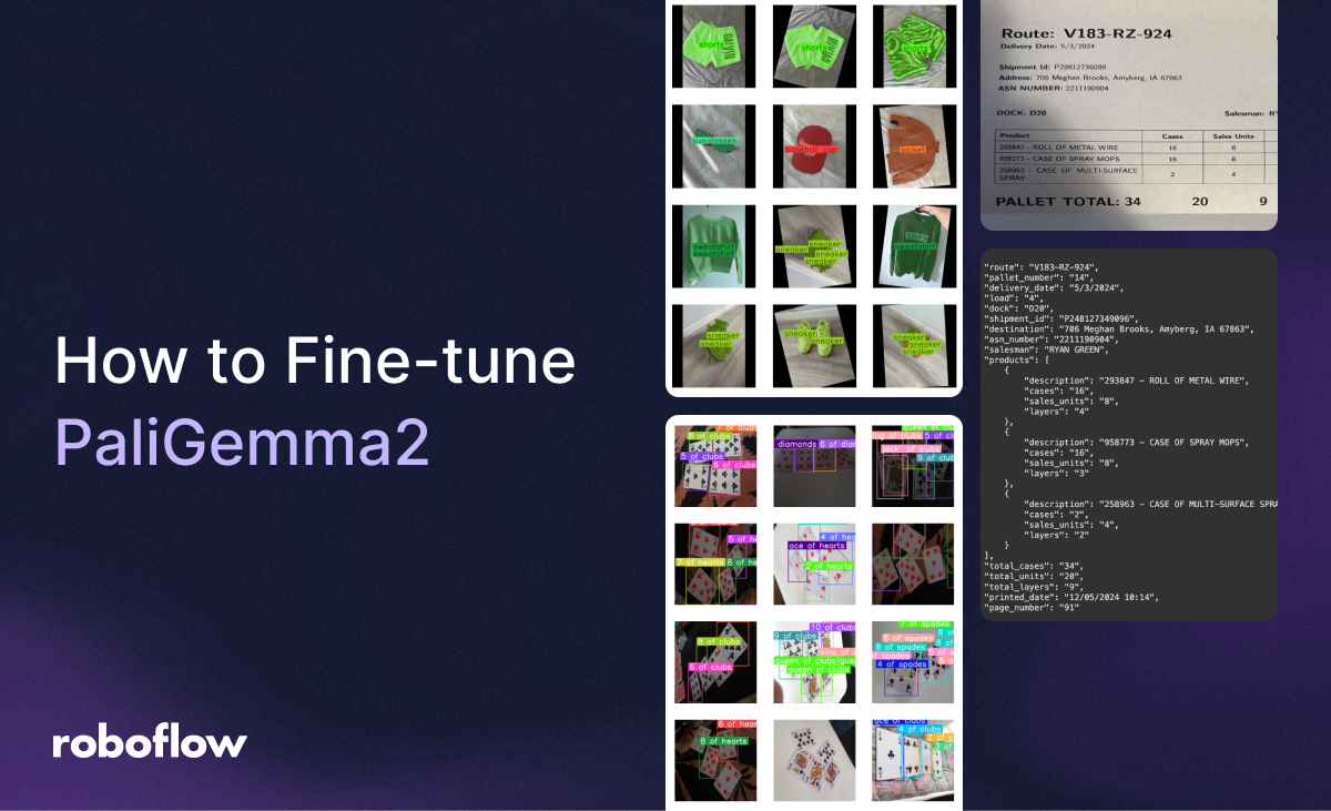
PaliGemma 2, released by Google on December 5th, 2024, is an updated and significantly enhanced version of the PaliGemma vision-language model (VLM) introduced earlier this year.

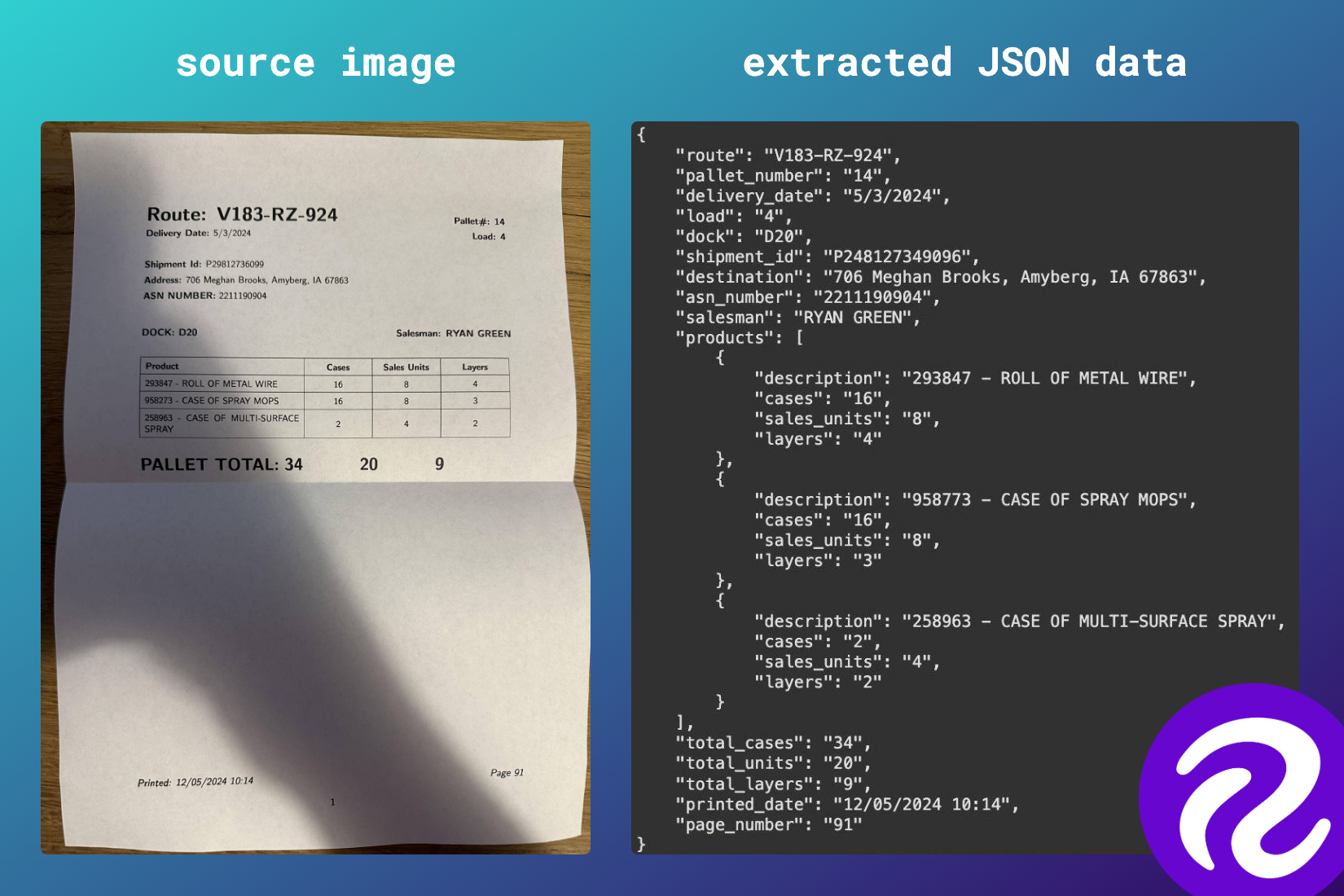
This tutorial will demonstrate how to fine-tune PaliGemma 2 using Google Colab to extract data from an image in JSON format. We will also provide some tips for fine-tuning for other vision-language tasks. Let’s get started!

What is PaliGemma 2?

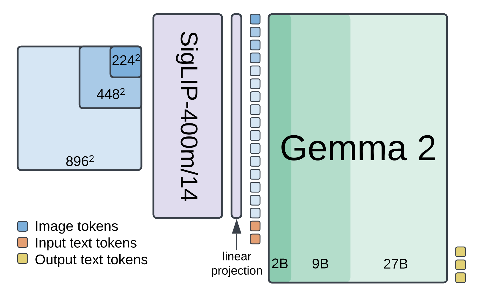
PaliGemma 2 combines a SigLIP-So400m vision encoder with a Gemma 2 language model to process images and text. The SigLIP-So400m encoder processes an image at various resolutions (224px, 448px, or 896px) and outputs a sequence of image tokens. These tokens are then linearly projected and combined with input text tokens.

Finally, the Gemma 2 language model, ranging in size from 2B to 27B parameters, processes these combined tokens and autoregressively generates output text tokens.

This architecture enables PaliGemma 2 to be fine-tuned for various tasks, including captioning, visual question answering (VQA), optical character recognition (OCR), object detection, and instance segmentation.

PaliGemma 2 Fine-tuning Expected Dataset Format

Annotate Data for PaliGemma 2 Fine-Tuning

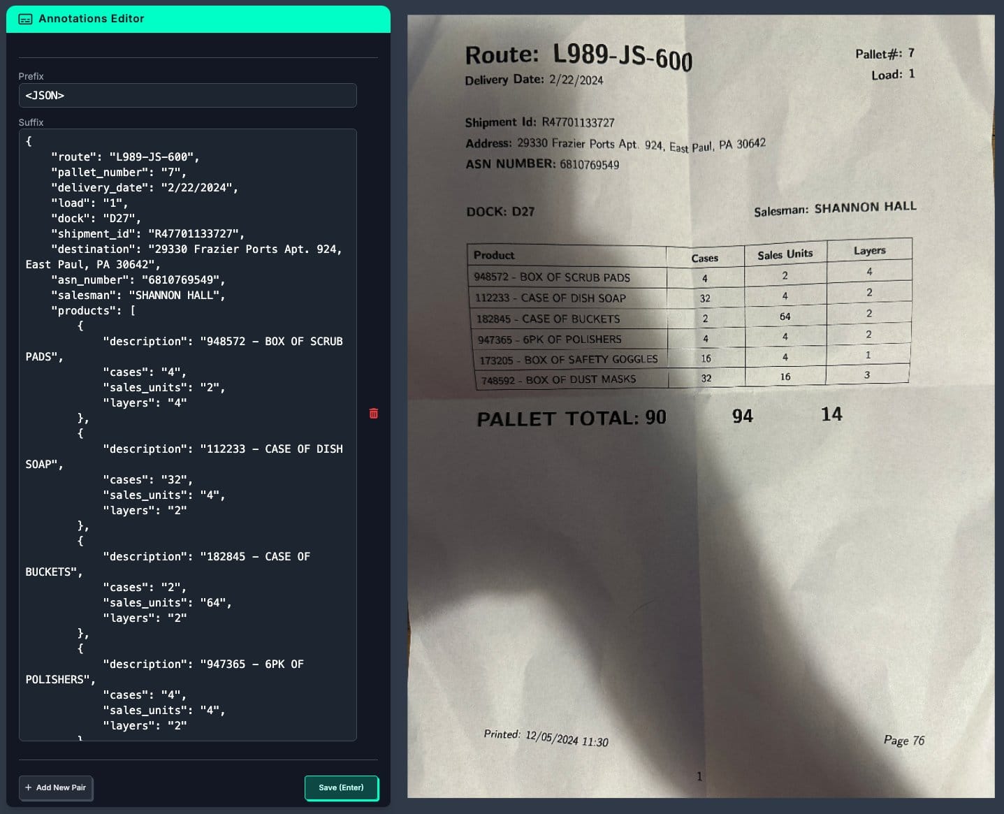
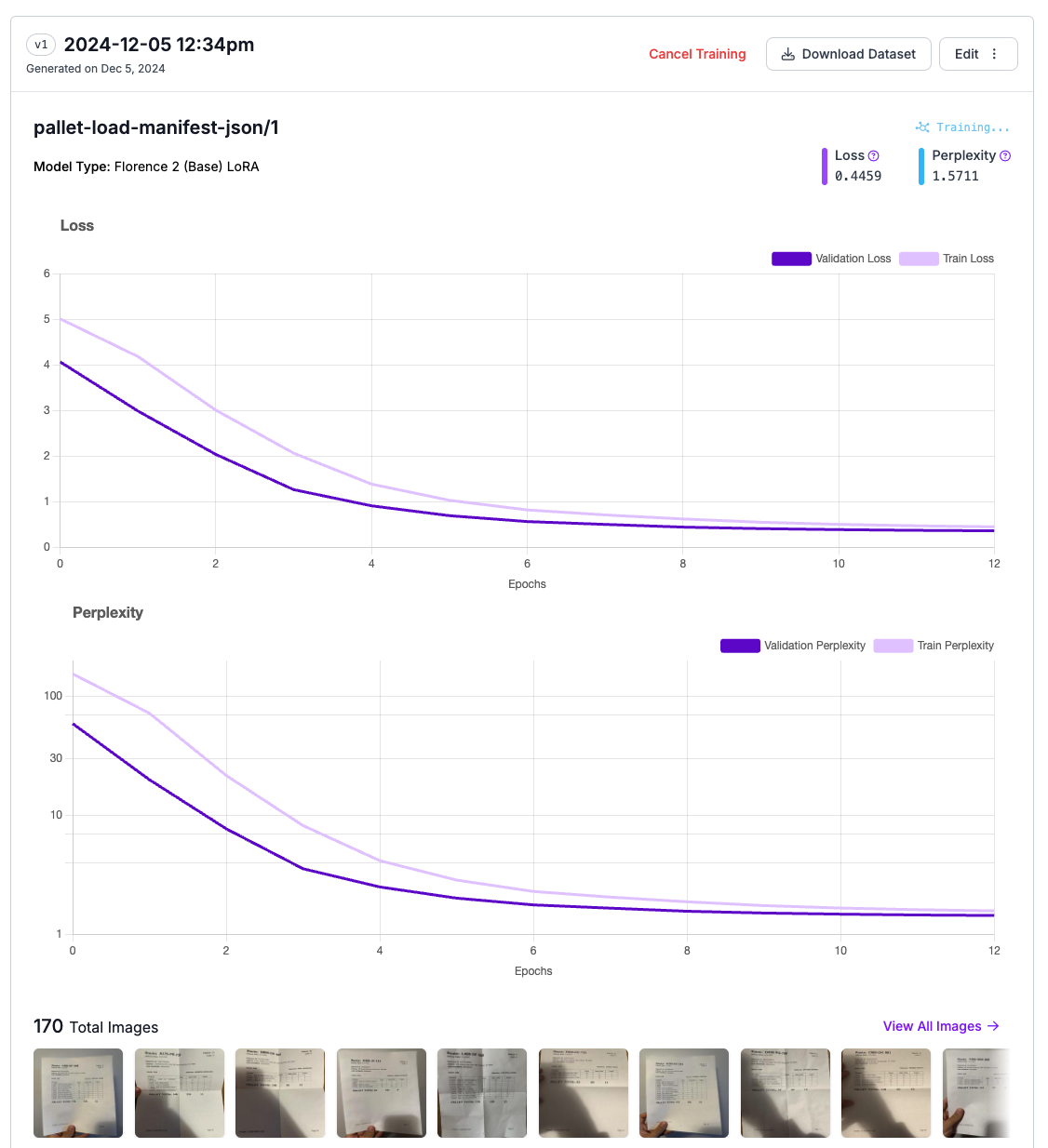
For this example, we'll train PaliGemma 2 to analyze pallet manifests, which are documents that provide detailed information about the contents of a shipment on a pallet. We used 50 such documents to create this dataset, allocating 30 to the training set, 10 to the validation set, and 10 to the test set.

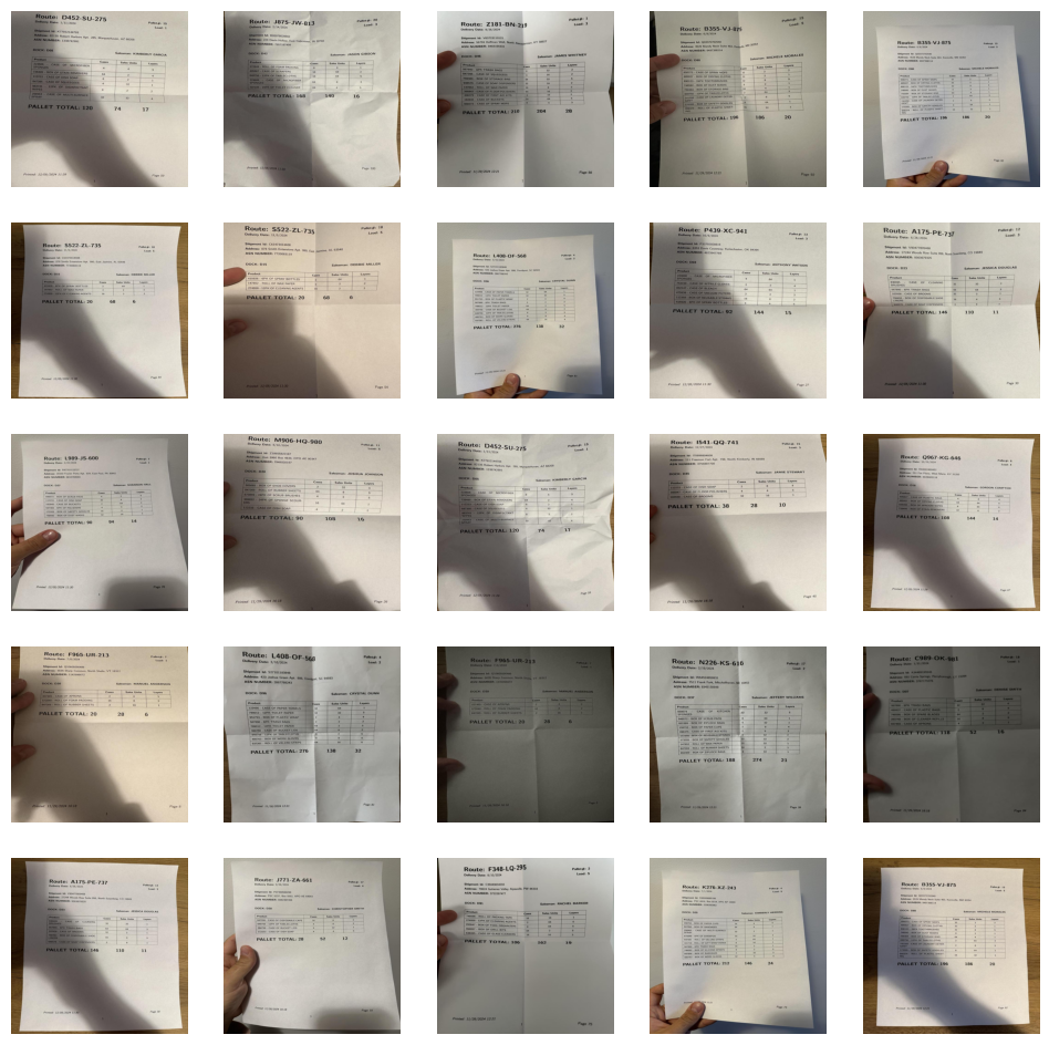
The documents in the training set were printed and then photographed at different angles, under various lighting conditions, and with varying degrees of damage. Each document in the training set was used 5 times, resulting in 150 images in the training set.  Each document in the test and validation sets was photographed once, but under different lighting conditions and with varying degrees of damage.  

The photos were then uploaded to Roboflow, where we created a multi-modal project and performed the annotations. The label at this point is a string representing a valid JSON containing all the information found on the document, such as route ID, shipment ID, delivery address, and product list.

Download Dataset in PaliGemma 2 Format

The dataset we prepared can be downloaded from Roboflow Universe using the roboflow package.

pip install roboflow

from roboflow import Roboflow

rf = Roboflow(api_key=ROBOFLOW_API_KEY)

project = rf.workspace("roboflow-jvuqo").project("pallet-load-manifest-json")
version = project.version(2)
dataset = version.download("jsonl")

The downloaded dataset has the following structure:

pallet-load-manifest-json/
├── train/
│   ├── train_image_1.png
│   ├── train_image_2.png
│   ├── ...
│   └── annotations.jsonl
├── test/
│   ├── test_image_1.png
│   ├── test_image_2.png
│   ├── ...
│   └── annotations.jsonl
└── valid/
    ├── valid_image_1.png
    ├── valid_image_2.png
    ├── ...
    └── annotations.jsonl

The downloaded dataset includes three subsets: train, test, and valid. Each subset contains images and an annotations.jsonl file. Regardless of the task, each dataset should be prepared in the JSONL format, where each line of the file is a valid JSON object. 

Each JSON object has three keys: image, prefix, and suffix. The image key holds the name of the image file associated with the data entry. The prefix key contains the prompt that will be sent to PaliGemma2, while the suffix key stores the expected output.

JSONL Dataset Loader

To utilize our dataset during training, we need to load it. We'll build a JSONLDataset class based on the PyTorch Dataset class, implementing the required methods.

import os
import json
from PIL import Image
from torch.utils.data import Dataset


class JSONLDataset(Dataset):
    def __init__(self, jsonl_file_path: str, image_directory_path: str):
        self.jsonl_file_path = jsonl_file_path
        self.image_directory_path = image_directory_path
        self.entries = self._load_entries()

    def _load_entries(self):
        entries = []
        with open(self.jsonl_file_path, 'r') as file:
            for line in file:
                data = json.loads(line)
                entries.append(data)
        return entries

    def __len__(self):
        return len(self.entries)

    def __getitem__(self, idx: int):
        if idx < 0 or idx >= len(self.entries):
            raise IndexError("Index out of range")

        entry = self.entries[idx]
        image_path = os.path.join(
            self.image_directory_path, entry['image'])
        image = Image.open(image_path).convert("RGB")
        return image, entry

Finally, we initialize three datasets for each of our subsets:

train_dataset = JSONLDataset(
    jsonl_file_path=f"{dataset.location}/train/annotations.jsonl", 
    image_directory_path=f"{dataset.location}/train"
) 

valid_dataset = JSONLDataset(
    jsonl_file_path=f"{dataset.location}/valid/annotations.jsonl", 
    image_directory_path=f"{dataset.location}/valid"
) 

test_dataset = JSONLDataset(
    jsonl_file_path=f"{dataset.location}/test/annotations.jsonl", 
    image_directory_path=f"{dataset.location}/test"
)

Chose PaliGemma 2 Baseline Checkpoint

PaliGemma 2 offers 9 pre-trained models with sizes of 3B, 10B, and 28B parameters, and resolutions of 224px, 448px, and 896px pixels. Choosing the appropriate baseline checkpoint is crucial for optimal performance and depends on several key factors:

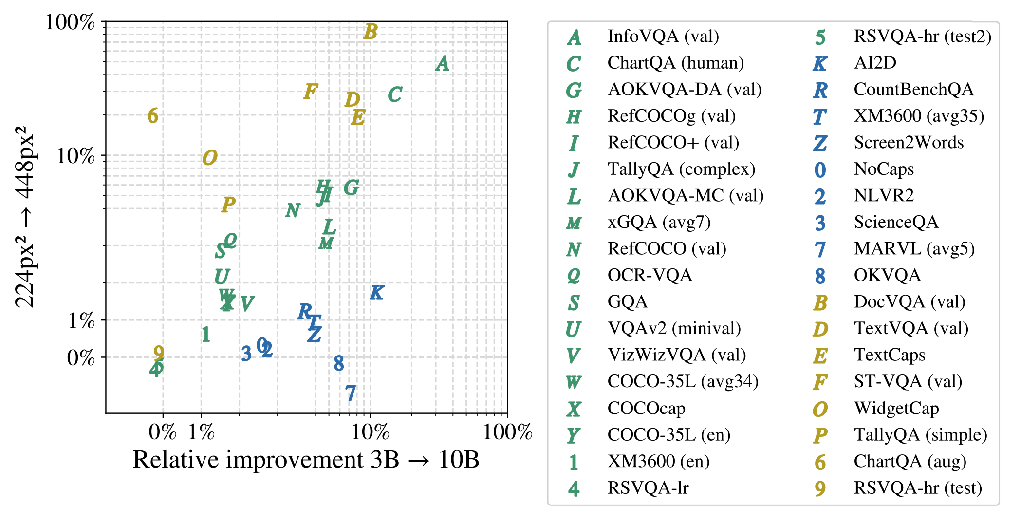
- Specific vision-language task: For tasks involving text, document, chart, or screen understanding, like ST-VQA, TallyQA, TextCaps, and TextVQA, prioritize higher resolution checkpoints (448px or 896px). These tasks benefit from the enhanced visual detail. If your task requires complex reasoning or multilingual capabilities, opt for checkpoints with larger language models (10B or 28B) even if it involves using a lower resolution.

- Available hardware: The table below provides insights into the relative training cost for various model sizes and resolutions. Increasing either factor significantly increases the computational demand. Select a checkpoint that aligns with your hardware's capabilities.

- Amount of data you have: Larger language models typically require more data for effective fine-tuning. Starting with a smaller model might be more appropriate if you have a limited dataset.

PaliGemma 2 Memory Optimizations

Fine-tuning large vision-language models like PaliGemma 2 can be resource-intensive. To put this into perspective, the largest variant of the recent YOLOv11 object detection model (YOLOv11x) has 56.9M parameters. In contrast, PaliGemma 2 models range from 3B to 28B parameters, making them significantly larger and more demanding to train. Employing memory optimization techniques is crucial for reducing costs associated with high-end hardware. Here are some strategies to consider:

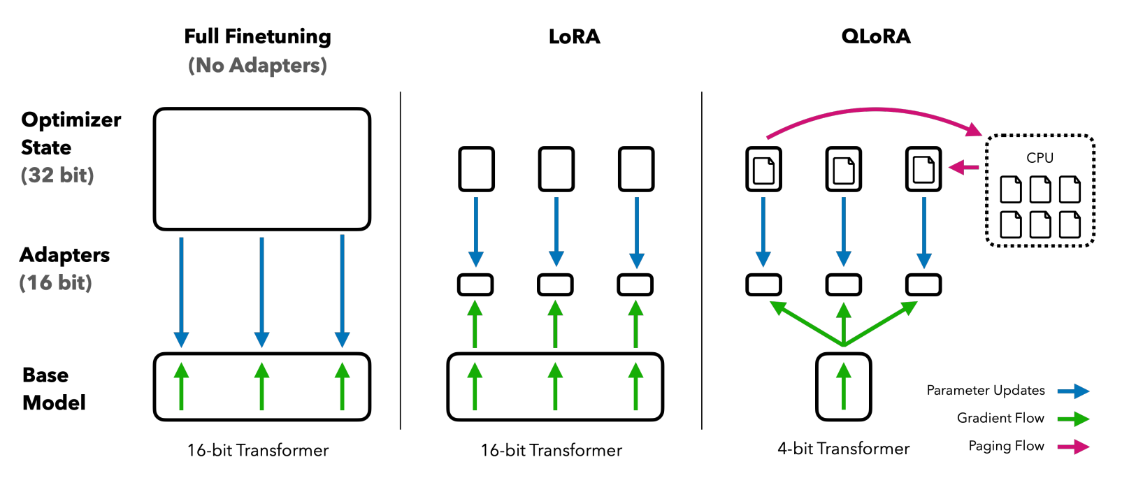
LoRA (Low-Rank Adaptation)

LoRA is a technique that makes fine-tuning large language models more efficient. Instead of adjusting all the parameters in the model, LoRA focuses on optimizing a smaller set of parameters. 

LoRA adds a smaller matrix to the large matrix representing the model's weights. This smaller matrix is easier to train and requires less memory. By adjusting only this smaller matrix, LoRA can effectively fine-tune the model while significantly reducing the memory footprint during training. 

This method often achieves performance close to full fine-tuning, where all parameters are adjusted, but with much less memory usage.

QLoRA (Quantized LoRA)

QLoRA combines LoRA with 4-bit quantization, further reducing memory usage. It quantizes the pre-trained model weights to 4-bit precision, keeping only the LoRA parameters in full precision. This allows for training even larger models on limited hardware.

Freezing the Vision Encoder

For tasks primarily focused on language processing with visual input, consider freezing the weights of the vision encoder (SigLIP). This prevents the vision encoder's weights from being updated during training, reducing the number of trainable parameters and memory requirements.

Load Pre-trained PaliGemma 2 Model

Before proceeding, ensure you have the necessary libraries installed by running the following command:

pip install -q peft bitsandbytes transformers>=4.47.0

Now, let's load the model using the following code:

import torch 
from peft import get_peft_model, LoraConfig
from transformers import PaliGemmaProcessor, PaliGemmaForConditionalGeneration, BitsAndBytesConfig

MODEL_ID ="google/paligemma2-3b-pt-224" 
DEVICE = torch.device("cuda" if torch.cuda.is_available() else "cpu")

processor = PaliGemmaProcessor.from_pretrained(MODEL_ID)

if USE_LORA or USE_QLORA: 
    lora_config = LoraConfig(
    r=8,
    target_modules=[
        "q_proj", 
        "o_proj", 
        "k_proj", 
        "v_proj", 
        "gate_proj", 
        "up_proj", 
        "down_proj"
    ],
    task_type="CAUSAL_LM",
    )
    if USE_QLORA:
        bnb_config = BitsAndBytesConfig(
        load_in_4bit=True,
        bnb_4bit_quant_type="nf4",
        bnb_4bit_compute_type=torch.bfloat16
            )
    model = PaliGemmaForConditionalGeneration.from_pretrained(
        MODEL_ID, 
        device_map="auto", 
        quantization_config=bnb_config if USE_QLORA else None,
        torch_dtype=torch.bfloat16)
    model = get_peft_model(model, lora_config)
    model = model.to(DEVICE)
    model.print_trainable_parameters()
else:
    model = PaliGemmaForConditionalGeneration.from_pretrained(
        MODEL_ID, device_map="auto").to(DEVICE)
    model = model.to(DEVICE)

    if FREEZE_VISION:
        for param in model.vision_tower.parameters():
            param.requires_grad = False

        for param in model.multi_modal_projector.parameters():
            param.requires_grad = False

TORCH_DTYPE = model.dtype

Train a PaliGemma 2 Model

Now that we've prepared our dataset and loaded the pre-trained PaliGemma 2 model, it's time to fine-tune it for our task. First, we define a collate_fn function to process our data before feeding it to the model:

from transformers import Trainer, TrainingArguments


def collate_fn(batch):
    images, labels = zip(*batch)

    paths = [label["image"] for label in labels]
    prefixes = ["<image>" + label["prefix"] for label in labels]
    suffixes = [label["suffix"] for label in labels]

    inputs = processor(
        text=prefixes,
        images=images,
        return_tensors="pt",
        suffix=suffixes,
        padding="longest"
    ).to(TORCH_DTYPE).to(DEVICE)

    return inputs

This function takes a batch of (image, label) pairs and prepares the inputs in the format expected by PaliGemma 2. This includes adding the <image> prefix to the text prompts and padding sequences to ensure consistent lengths within the batch.

Next, we define the training arguments:

args = TrainingArguments(
    num_train_epochs=3,
    remove_unused_columns=False,
    per_device_train_batch_size=3,
    gradient_accumulation_steps=16,
    warmup_steps=2,
    learning_rate=5e-5,
    weight_decay=1e-6,
    adam_beta2=0.999,
    logging_steps=200,
    optim="paged_adamw_8bit" if USE_QLORA else "adamw_hf",
    save_strategy="steps",
    save_steps=1000,
    save_total_limit=1,
    output_dir="paligemma2_json_extraction",
    bf16=True,
    report_to=["tensorboard"],
    dataloader_pin_memory=False
)

Here are some key hyperparameters:

- num_train_epochs: The number of times the model will iterate over the entire training dataset. Increasing this value may improve performance but also increase training time and potentially lead to overfitting.

- per_device_train_batch_size: The number of training examples used in each iteration on each device. Increasing this value can improve training speed and stability, but it requires more memory.

- gradient_accumulation_steps: The number of steps to accumulate gradients before performing a weight update. This effectively increases the batch size without requiring more memory. Increasing this value can improve stability with smaller batch sizes but may slow down training.

- learning_rate: Controls the step size taken during optimization. Increasing this value may speed up learning but can lead to instability or overshooting the optimal solution.

- weight_decay: A regularization technique that prevents overfitting by adding a penalty to the model's weights. Increasing this value can help prevent overfitting but may also limit the model's ability to learn complex patterns.

Finally, we create a Trainer instance and start the training process:

trainer = Trainer(
    model=model,
    train_dataset=train_dataset,
    eval_dataset=valid_dataset,
    data_collator=collate_fn,
    args=args
)
trainer.train()

This will fine-tune our PaliGemma 2 model on the provided dataset. Remember to monitor the training process and adjust the hyperparameters as needed to achieve optimal performance.

Run Inference with Fine-tuned PaliGemma 2 Model

After completing the training process, we can use our fine-tuned PaliGemma 2 model to make predictions on new images.

image, label = test_dataset[0]
prefix = "<image>" + label["prefix"]
suffix = label["suffix"]

inputs = processor(
    text=prefix,
    images=image,
    return_tensors="pt"
).to(TORCH_DTYPE).to(DEVICE)

# Calculate the length of the input sequence
prefix_length = inputs["input_ids"].shape[-1]  

with torch.inference_mode():
    generation = model.generate(
        **inputs, max_new_tokens=256, do_sample=False, num_beams=3)
    
    # Extract only the generated tokens by slicing the sequence
    generation = generation[0][prefix_length:]  
    
    generated_text = processor.decode(
        generation, skip_special_tokens=True)

This code snippet takes an image and its corresponding label from the test dataset. It then prepares the input for the model by adding the <image> prefix and encoding it using the processor.

The model.generate() function then generates a sequence of token IDs. This sequence contains the IDs of both the input tokens and the generated ones. To get only the generated output, we need to remove the input token IDs. We do this by slicing the generation tensor starting from prefix_length  — this way, we drop the input IDs and keep only the generated ones.

Finally, we decode these generated token IDs into text using the processor, giving us the model's prediction.

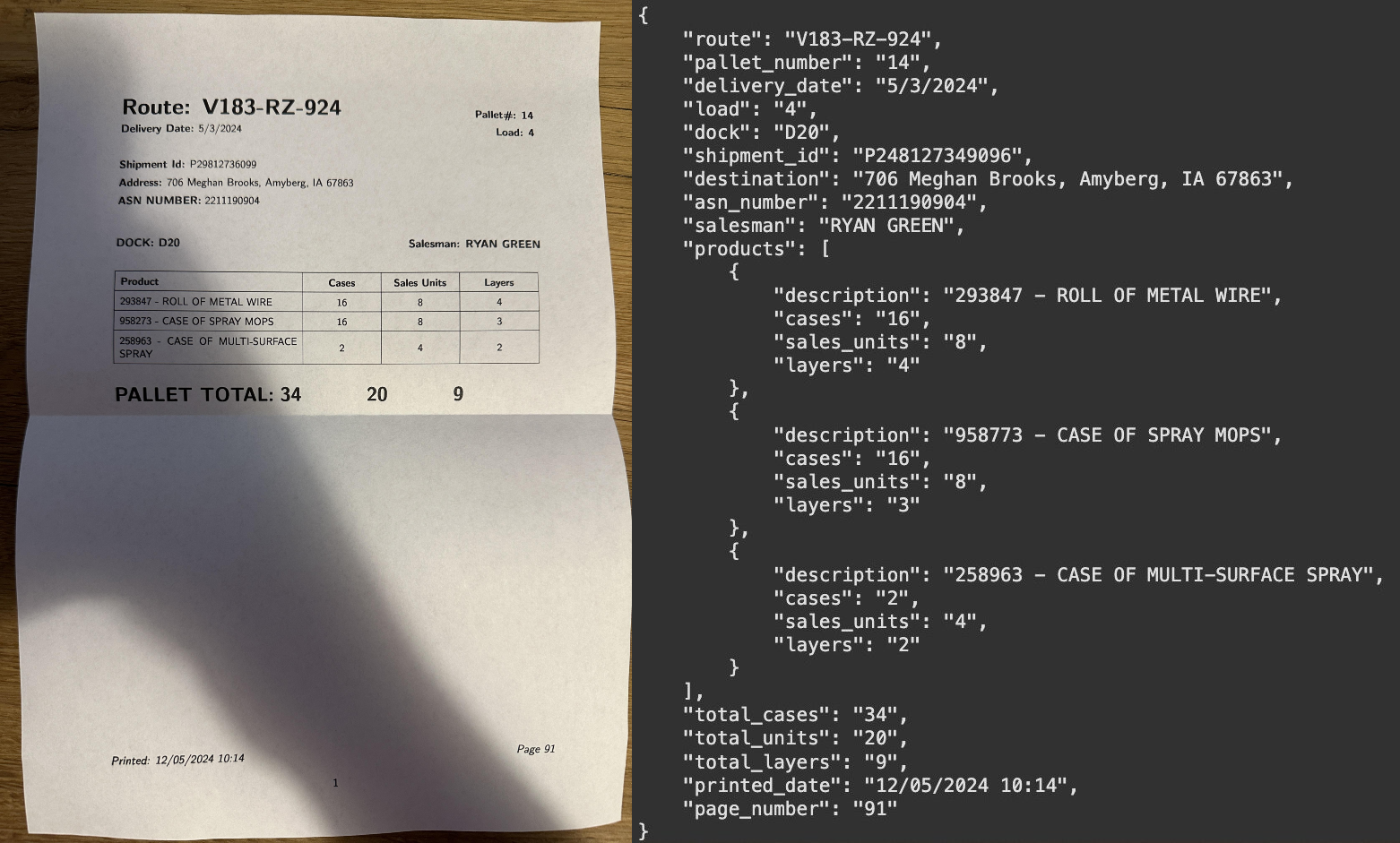
You can compare the generated_text with the suffix (ground truth) to evaluate the quality of the predictions. For this comparison, you can use metrics like BLEU score, ROUGE score, or METEOR score, which measure the similarity between the generated text and the ground truth. It's also helpful to visualize the image and the predicted output to gain a better understanding of the model's performance.

Extra: Preparing Data for PaliGemma 2 Object Detection Training

To fine-tune PaliGemma 2 for object detection, the overall structure of the dataset remains the same, but the prefix and suffix fields within the JSONL files require adjustments. 

In the prefix, use the keyword detect followed by a semicolon-separated list of the object classes you want to detect. For example, detect person; car; bicycle. The suffix should contain the detection results, with each object represented by its bounding box and class name. The bounding box is formatted as <loc{Y1}><loc{X1}><loc{Y2}><loc{X2}>, where X1, Y1, X2, and Y2 are the normalized coordinates of the top-left and bottom-right corners of the box, respectively. These coordinates are normalized to an image size of 1024x1024 and each value should have 4 digits (padded with zeros if necessary).

The Gemma2 tokenizer has been enhanced with 1024 additional tokens (<loc0000> to <loc1023>) to represent these normalized image-space coordinates.

Conveniently, all object detection datasets on Roboflow Universe can be exported in a PaliGemma 2-compatible format. You can use the following code snippet to download a dataset in this format:

from roboflow import Roboflow

rf = Roboflow(api_key=ROBOFLOW_API_KEY)

project = rf.workspace("roboflow-jvuqo").project("poker-cards-fmjio")
version = project.version(4)
dataset = version.download("paligemma")

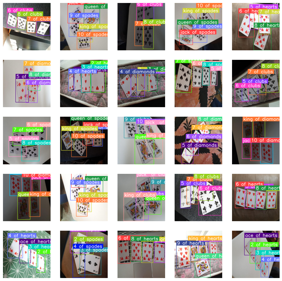
For a detailed walkthrough of the object detection fine-tuning process, refer to our PaliGemma object detection fine-tuning tutorial recorded a few months ago. This tutorial provides a step-by-step guide to fine-tuning PaliGemma 2 for object detection, including data preparation, model training, and evaluation.

We also have a dedicated notebook that demonstrates the fine-tuning process for PaliGemma 2.

Extra: Preparing Data for PaliGemma 2 Instance Segmentation Training

Fine-tuning PaliGemma2 for instance segmentation requires a slightly different approach to data preparation. In addition to the standard image and annotation data, we utilize a specialized encoding scheme for the segmentation masks.

Gemma2's encoder has been expanded with 128 new entries (<seg000> to <seg127>) representing codewords. These codewords are used by a lightweight referring-expression segmentation vector-quantized variational auto-encoder (VQ-VAE) to efficiently represent segmentation masks. This VQ-VAE model acts as a separate, smaller model solely for converting annotation masks into text labels.

The VQ-VAE model is part of the big_vision repository (home of PaliGemma and other related models) and can be loaded as follows:

from big_vision.pp.proj.paligemma.segmentation import get_checkpoint checkpoint = 

get_checkpoint(model='oi')

You can find detailed setup instructions for big_vision, along with an end-to-end instance segmentation fine-tuning example, in the linked notebook.

Assuming you've downloaded your dataset in COCO format using the following code:

from roboflow import Roboflow

rf = Roboflow(api_key=ROBOFLOW_API_KEY)

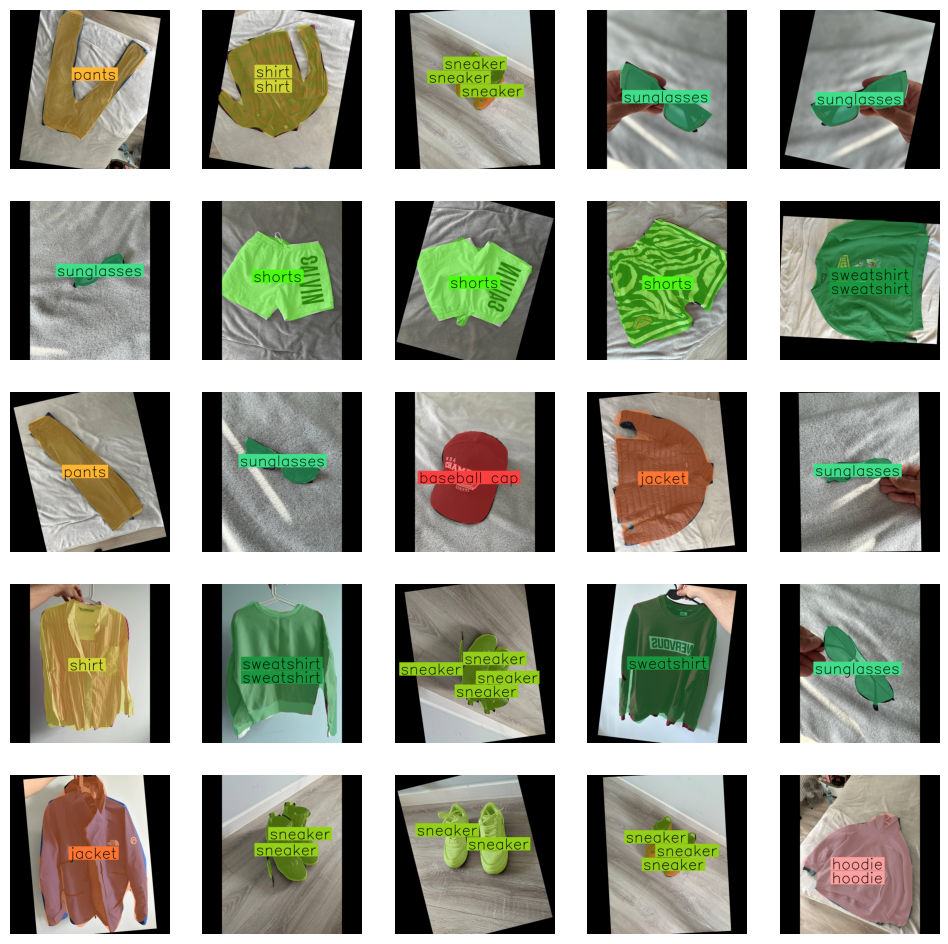
project = rf.workspace("roboflow-jvuqo").project("fashion-assistant-segmentation")
version = project.version(5)
dataset = version.download("coco-segmentation")

You can use the code below to convert the COCO segmentation labels into a JSONL dataset compatible with PaliGemma2. This code snippet iterates through the dataset, extracts the bounding boxes and masks for each object, encodes the masks using the VQ-VAE, and formats the data into the required prefix and suffix structure.

import os
import numpy as np
import tensorflow as tf
import supervision as sv

from big_vision.pp.proj.paligemma.segmentation import encode_to_codebook_indices, get_checkpoint

# Load the VQ-VAE checkpoint
checkpoint = get_checkpoint(model='oi') 

# Load the dataset in COCO format
ds = sv.DetectionDataset.from_coco(
    images_directory_path=f"{dataset_path}",
    annotations_path=f"{dataset_path}/_annotations.coco.json",
    force_masks=True
)

# Define the segmentation and location tokens
seg_tokens = tf.constant(['<seg%03d>' % i for i in range(128)])
loc_tokens = tf.constant(['<loc%04d>' % i for i in range(1024)])

labels = []
prefix = "segment " + " ; ".join(ds.classes)  # Construct the prefix with class names

for image_path, image, annotations in ds:
    h, w, _ = image.shape
    image_name = os.path.basename(image_path)
    suffix_components = []

    # Skip if annotations are missing
    if annotations.xyxy is None or annotations.mask is None or annotations.class_id is None:  
        continue

    for xyxy, mask, class_id in zip(annotations.xyxy, annotations.mask, annotations.class_id):
        y1 = tf.cast(tf.round(xyxy[1]), tf.int32)
        x1 = tf.cast(tf.round(xyxy[0]), tf.int32)
        y2 = tf.cast(tf.round(xyxy[3]), tf.int32)
        x2 = tf.cast(tf.round(xyxy[2]), tf.int32)

        mask = tf.convert_to_tensor(mask.astype(np.uint8), dtype=tf.uint8)

        # Resize the mask to 64x64
        mask = tf.image.resize(
            mask[None, y1:y2, x1:x2, None],
            [64, 64],
            method='bilinear',
            antialias=True,
        )

        # Encode the mask using the VQ-VAE
        mask_indices = encode_to_codebook_indices(checkpoint, mask)[0]  
        mask_string = tf.strings.reduce_join(tf.gather(seg_tokens, mask_indices))

        # Normalize bounding box coordinates
        bbox = xyxy[[1, 0, 3, 2]] / np.array([h, w, h, w])  
        binned_loc = tf.cast(tf.round(bbox * 1023), tf.int32)
        binned_loc = tf.clip_by_value(binned_loc, 0, 1023)
        loc_string = tf.strings.reduce_join(tf.gather(loc_tokens, binned_loc))

        # Construct the suffix with bounding box and mask information
        suffix = tf.strings.join([loc_string, mask_string])  
        suffix = f"{suffix.numpy().decode('utf-8')} {ds.classes[class_id]}"
        suffix_components.append(suffix)

    suffix = " ; ".join(suffix_components)
    labels.append({
        "image": image_name,
        "prefix": prefix,
        "suffix": suffix
    })

Conclusion

This tutorial provided a comprehensive guide to fine-tuning PaliGemma 2 for extracting JSON data from images. We addressed key steps including dataset preparation in the JSONL format, efficient model loading with techniques like LoRA and QLoRA, and the training process. 

PaliGemma 2's architecture, combining a vision encoder with a language model, enables adaptation to diverse tasks through fine-tuning. The availability of various model sizes and resolutions allows for selecting a checkpoint that balances performance with computational constraints.

Further examples of fine-tuning PaliGemma 2 for tasks such as object detection, LaTeX OCR, and more can be found in the accompanying notebooks. These resources demonstrate how to leverage PaliGemma 2's capabilities for different computer vision problems. For streamlined training and experimentation with VLMs, consider utilizing tools like Roboflow and the open-source maestro package.