
Image augmentation increases effective training set size by applying random transformations to existing images, but knowing how much to augment and which transforms to apply depends on your dataset. This experiment tests three variables across three public datasets of different sizes (26, 196, and 665 images of packages, raccoons, and potholes): augmentation type, augmentation count, and original dataset size. The results show no universal rule: for larger datasets, adding augmentations sometimes hurt model performance, while smaller datasets generally benefited, suggesting augmentation strategy should be tuned rather than applied by default.
One of the amazing things about computer vision is using existing images plus random changes to increase your effective sample size. Suppose you have one photo containing a coffee mug. Then, copy that photo and rotate it 10 degrees clockwise. From your point of view, you haven’t done very much.
But you’ve (really easily) doubled the number of images you’re about to give your model! Your computer vision model now gets a whole new perspective on what that coffee mug looks like.
Now creating two versions of the same existing photo of a coffee mug isn’t quite as good as taking two actual separate pictures of a coffee mug. You shouldn’t, for example, take one photo and augment it 10,000 times and fit an object detection model on that data, then expect your model to perform as well as if you had taken 10,000 real pictures of a coffee mug. There are some limitations to image augmentation.
That said, image augmentation is a really powerful technique to generate new data from existing data. A huge benefit to using Roboflow is that you can do this with one click of a button!
Just how powerful is image augmentation? I decided to run a little experiment. I explored how model performance shifted based on three different dimensions: size of the original dataset, type of augmentations, and number of augmentations.
Size of the original dataset
I selected three public image datasets from public.roboflow.com. (You can use these datasets yourself right now!)
- A packages dataset, consisting of 26 images of packages located near the doors of apartments and homes.
- A raccoons dataset, consisting of 196 images of raccoons.
- A potholes dataset, consisting of 665 images of potholes on the road.
Type of augmentations
At the beginning of the article, I used rotate as an example augmentation: copy an image and rotate it 10 degrees. However, there are many different types of image augmentation techniques! I broke the types of augmentations I explored into three sets. (Why break the augmentations into sets? Well, Roboflow enables you to apply up to 23 different augmentation techniques! Doing an exhaustive search of those would take a long time.)
Set A: Random rotate, random crop, and random noise
- Random rotate: For each augmentation, I randomly rotated each image by up to 10 degrees counterclockwise or clockwise.
- Random crop: For each augmentation, I randomly cropped each image by up to 20%. You can think of this as zooming in on the image.
- Random noise: For each augmentation, I randomly added black or white pixels to 10% of the pixels in the image. It looks like I sprinkled salt and pepper over the image, which can help protect against adversarial attacks and prevent overfitting.
Set B: Random brightness, random blur, and random cutout, plus all “Set A” augmentations
- Random brightness: For each augmentation, I randomly brightened or darkened the image by up to 30%. For an image, it’s almost like if the sun were really bright or if it were a really cloudy day.
- Random blur: For each augmentation, I added random Gaussian blur of up to 1.75 pixels, which can simulate a camera moving like if you’re taking a picture while riding in a vehicle.
- Random cutout: For each augmentation, I added 5 randomly-located black boxes on the image of up to 15% of the image. This replicates occlusion, where an object of interest is blocked by another object from the camera’s view.
Set C: Bounding box-level rotation, bounding box-level crop, and bounding box-level brightness, plus all “Set A” and “Set B” augmentations.
Bounding box-level augmentations are like regular image augmentations, except instead of the entire image changing (which is what happens with image augmentation), only the area in the bounding box changes is affected by these. They were popularized by a 2019 Google research paper.
- Random bounding box-level rotation: For each augmentation, I randomly rotated the content in each bounding box by up to 10 degrees counterclockwise or clockwise.
- Random bounding box-level crop: For each augmentation, I randomly cropped the content in each bounding box by up to 20%.
- Random bounding box-level brightness: For each augmentation, I randomly brightened or darkened the bounding box region of the image by up to 30%.
Number of augmentations
For each image, we augment (copy and add random changes to) that image a certain number of times. One of the main things we want to understand is, how does the number of augmentations affect model performance?
For each dataset, we construct an augmented dataset by augmenting each image a certain number of times, then fit a model on each augmented dataset.
- 0x augmentation -- this is just the regular dataset without augmentation
- 3x augmentation -- each image is copied 3 times with random perturbations
- 5x augmentation
- 10x augmentation
- 20x augmentation
Measuring performance
We measured performance by looking at three common metrics in object detection:
- Mean average precision (mAP): the gold standard metric. mAP ranges from 0% to 100%. The closer your mAP is to 100%, the better your model performs.
- Precision: Not to be confused with mean average precision, precision (also called positive predictive value) calculates the number of correctly predicted objects divided by the total number of objects predicted by the model. As an example, if a model predicts that there are 10 objects across a dataset and 8 of those predictions are correct, our model has an 80% precision score on that dataset.
- Recall: Also called sensitivity, recall calculates the number of correctly predicted objects divided by the total number of “ground truth” objects in the data. As an example, if a model predicts there are 20 objects in a dataset and our model correctly detects 8 of those objects, our model has a 40% (8/20) recall score on that dataset.
Results
Packages Dataset
When fitting models on the packages dataset (with 26 source images), the mAP was extremely low before augmenting the images – 3.5% out of a potential 100%. Applying augmentation techniques significantly increased the mAP by as high as 80 percentage points.
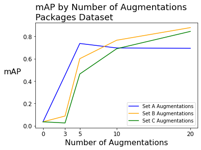
We see similar improvement with precision and recall, going from 0% with zero augmentations up to above 70% or 80%. The full table of mAP, precision, and recall scores for the packages dataset is below.
| set A | set A | set A | set B | set B | set B | set C | set C | set C | |
|---|---|---|---|---|---|---|---|---|---|
| packages (n=26) | mAP | precision | recall | mAP | precision | recall | mAP | precision | recall |
| No augmentation | 3.50% | 0% | 0% | 3.50% | 0% | 0% | 3.50% | 0% | 0% |
| 3x augmentation | 45.30% | 10.80% | 50.00% | 8.70% | 100% | 7.10% | 2.50% | 0% | 0% |
| 5x augmentation | 73.60% | 61.40% | 78.60% | 60.00% | 11.60% | 71.40% | 46.30% | 20.00% | 57.10% |
| 10x augmentation | 69.60% | 34.70% | 78.60% | 76.50% | 42.10% | 78.60% | 68.90% | 30.70% | 71.40% |
| 20x augmentation | 69.30% | 72.50% | 64.30% | 87.80% | 87% | 71.40% | 84.40% | 75.50% | 66.10% |
Raccoons Dataset
When fitting models on the raccoons dataset (with 196 source images), the mean average precision was above 88% with zero augmentations. In this case, the effect of augmentations varied!
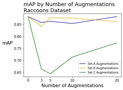
The non-bounding box-level augmentations had no significant effect on mAP, though there was significant improvement (up to 20 or 30 percentage points) in the precision.
Bounding box-level augmentations had a significantly negative impact on mAP and recall.
| set A | set A | set A | set B | set B | set B | set C | set C | set C | |
|---|---|---|---|---|---|---|---|---|---|
| Dataset 2: raccoons (n=196) | mAP | precision | recall | mAP | precision | recall | mAP | precision | recall |
| No augmentation | 88.20% | 47.80% | 90.50% | 88.20% | 47.80% | 90.50% | 88.20% | 47.80% | 90.50% |
| 3x augmentation | 85.70% | 58.50% | 83.30% | 84.10% | 52.80% | 88.10% | 66.30% | 46.00% | 73.80% |
| 5x augmentation | 86.20% | 69.70% | 88.10% | 87.70% | 78.60% | 88.10% | 64.30% | 43.50% | 73.80% |
| 10x augmentation | 85.30% | 73.40% | 82.10% | 87.50% | 59.90% | 90.50% | 71.30% | 45.10% | 78.60% |
| 20x augmentation | 88.20% | 62.10% | 90.50% | 86.10% | 65.20% | 84.90% | 77.20% | 49.60% | 85.70% |
Potholes Dataset
When fitting models on the potholes dataset (with 665 source images), the mAP began around 74% with zero augmentations.
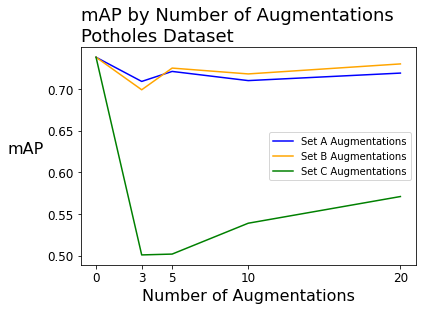
After augmenting the potholes dataset, we see performance effects that were similar to the raccoons dataset. The raccoons and potholes datasets had significantly more source images (196 and 665, respectively) than the packages dataset (26 images).
| set A | set A | set A | set B | set B | set B | set C | set C | set C | |
|---|---|---|---|---|---|---|---|---|---|
| Dataset 3: potholes (n=665) | mAP | precision | recall | mAP | precision | recall | mAP | precision | recall |
| No augmentation | 73.80% | 46.70% | 78.70% | 73.80% | 46.70% | 78.70% | 73.80% | 46.70% | 78.70% |
| 3x augmentation | 70.90% | 49.50% | 75.20% | 69.90% | 53.30% | 74.80% | 50.10% | 51.00% | 51.80% |
| 5x augmentation | 72.10% | 57.70% | 73.00% | 72.50% | 42.10% | 78.50% | 50.20% | 52.50% | 52.10% |
| 10x augmentation | 71.00% | 54.90% | 73.00% | 71.80% | 49.00% | 73.90% | 53.90% | 60.10% | 53.90% |
| 20x augmentation | 71.90% | 45.40% | 78.50% | 73.00% | 53.30% | 75.40% | 57.10% | 54.40% | 56.40% |
Takeaways
- The positive effects of augmentations seem to be most pronounced on datasets with small sample sizes. This is really good news: even if your dataset is really small, image augmentation can help your models perform reasonably well! The packages dataset, with 26 images, saw mAP improve by over 80 percentage points with augmentations!
- If you’re going to do augmentations, do more augmentations! While having 3 or 5 augmentations is helpful, you’ll often see a benefit if you increase your number of augmentations. For example, the mAP was always higher with 20 augmentations than with 3, and this was almost always true for precision and recall as well.
- More types of augmentations aren't always better. Bounding box-level augmentation techniques, when used in conjunction with non bounding box-level augmentation techniques, often had a negative impact on model performance. Subject-matter expertise and knowing which type of augmentation to apply in a given scenario is important!
- Augmentations aren’t magic. It's not as simple as "augmentations make things better." In a number of scenarios (where the sample size was already substantial), it was actually better to have zero augmentations than to augment the images. This might boil down to the specific images in the dataset or the specific types of augmentations that were selected. Computer vision is not a perfect science, but is also an art.
Note that each of the datasets contains exactly one class (packages, raccoons, and potholes, respectively). This isn’t always the case in object detection problems -- for example, the doors could be labeled in the packages dataset, so we’d include “packages” and “doors” as two separate classes.
So why did we only explore single-class object detection problems? Well, I’m already comparing a lot of variables here (size of the original dataset, number of augmentations, type of augmentations), so I opted to not also explore how the number of augmentations the impact of the number of classes. (Perhaps there’ll be a sequel blog post -- interested in writing one?)
To juice your models even more, consider using transfer learning and the types of augmentation we didn't explore in this post. Happy building!
Cite this Post
Use the following entry to cite this post in your research:
Matt Brems. (May 3, 2021). The power of image augmentation: an experiment. Roboflow Blog: https://blog.roboflow.com/the-power-of-image-augmentation-experiment/