Fastest Object Detection Models in 2026

Object detection has become one of the most widely used computer vision tasks in production. It is used to detect defects on manufacturing lines, identify vehicles in traffic systems, monitor inventory on shelves, inspect infrastructure, count objects in aerial imagery, and power real-time AI applications on edge devices. Speed is often the deciding factor when you move an object detection model to production line. The question is no longer only:

“Which object detection model is the most accurate?”

but, for real-world applications, the better question is:

Which object detection model gives the best accuracy at the lowest practical latency on my hardware?

A model that is highly accurate but too slow may not work for video analytics, robotics, drones, manufacturing inspection, or live monitoring. A model that is extremely fast but misses important objects may also fail in production. The best model is usually the one that gives the strongest balance between speed, accuracy, deployment simplicity, and performance on your own dataset.

In this guide, I will compare the fastest object detection models available this year, with a focus on models benchmarked and supported in the Roboflow ecosystem. My choice of models that I will cover are RF-DETR, YOLO26, Roboflow 3.0, YOLOv12, YOLO11, RT-DETR/RT-DETRv2, and RTMDet.

What Does Fastest Model Mean?

The fastest model is not always the model with the highest FPS or the lowest latency number. A model should be considered fast only if it can make predictions quickly while still detecting objects accurately.

Speed is usually measured using latency, which means the time taken to process one image. Lower latency means the model can process more frames per second. This is important for real-time applications such as video analytics, robotics, drones, factory inspection, and edge AI systems.

Accuracy is usually measured using object detection metrics such as AP50 and AP50:95. AP50:95 is stricter because it checks how well predicted boxes match real objects across multiple IoU thresholds.

Here by stating “fastest object detection models”, I mean models that provide the best practical balance between:

• Low inference latency
• Strong detection accuracy
• Real-time performance
• Practical deployment needs

Here I compare models using a practical speed-and-accuracy approach, considering single-image latency, COCO AP metrics, and RF100-VL generalization results.

Fastest Object Detection Models in 2026

Now let's see some popular fastest object detection models.

RF-DETR

RF-DETR should be the first model to consider when you need both high speed and strong accuracy. RF-DETR uses a transformer-based detection approach designed to work well across diverse datasets and deployment environments. In the benchmark data, RF-DETR variants form a strong accuracy-latency curve across different model sizes. The Nano, Small, and Medium variants are especially useful for real-time applications where latency matters but accuracy cannot be sacrificed too much.

RF-DETR is designed as an end-to-end detector. In many traditional object detection models, predictions are followed by post-processing steps such as Non-Maximum Suppression. NMS removes duplicate boxes, but it adds extra computation and can make deployment pipelines more complex. RF-DETR avoids this traditional post-processing-heavy structure. Its transformer-based architecture predicts objects directly, which helps simplify inference and reduce overhead. RF-DETR also benefits from strong visual backbones and architecture search, giving it strong accuracy without sacrificing real-time performance.

YOLO26

YOLO26 is another important object detection model family in 2026. It is part of the YOLO lineage, which has been popular for many years because of its speed, simplicity, and strong ecosystem support. YOLO26 is designed as a modern real-time vision model family. It supports object detection and other computer vision tasks, and it is available in multiple sizes from Nano to Extra Large.

One of the biggest improvements in YOLO26 is that it removes Non-Maximum Suppression from the prediction pipeline. This makes YOLO26 suitable for low-latency deployment because it reduces post-processing overhead. YOLO26 is also optimized for edge and low-power hardware.

Roboflow 3.0

Roboflow 3.0 is an object detection model with a strong balance of speed, accuracy, and deployment efficiency inside the Roboflow ecosystem. It offers different model size options, including Fast, Accurate, Medium, Large, and Extra Large. Roboflow 3.0 can be trained on custom datasets in Roboflow Train and deployed with Roboflow Inference, Workflows, Hosted API, or other Roboflow deployment options. This makes it another useful model to include when comparing fast object detection models for your own use case. This model can be used as alternative to various YOLO mdels.

YOLOv12

YOLOv12 is a YOLO-family object detection model. The model keeps the familiar YOLO-style workflow while adding architectural improvements focused on better accuracy and low-latency inference. YOLOv12 is a good model to include in a fastest object detection comparison because it improves on earlier YOLO-style detectors and remains practical for real-time use cases. However, for new projects in 2026, it should be treated as a strong comparison model rather than the default first choice. RF-DETR and YOLO26 are usually better starting points when you want the strongest current speed-accuracy tradeoff in the Roboflow ecosystem.

YOLO11

YOLO11 is a real-time computer vision model from the Ultralytics YOLO family. YOLO11 remains a useful baseline in 2026 because it is widely adopted, easy to train on custom datasets, and familiar to many computer vision teams. Although newer models such as RF-DETR and YOLO26 may offer stronger speed-accuracy tradeoffs, YOLO11 is still valuable for teams that already use YOLO-based training scripts, model exports, deployment pipelines, or edge workflows.

RT-DETR and RT-DETRv2

RT-DETR and RT-DETRv2 are important because they helped make transformer-based object detection more practical for real-time applications. Traditional DETR-style models were often accurate but slow to train or deploy. Real-time DETR models improved this by making transformer detection more efficient. In 2026, RT-DETR and RT-DETRv2 are best seen as important transformer detector baselines. However, RF-DETR is usually the stronger first choice in the Roboflow ecosystem because of its strong benchmark results, model variants, and deployment support.

RTMDet

RTMDet is another efficient real-time detector. It is useful in high-throughput scenarios where speed is very important. RTMDet has been used as a strong real-time object detection architecture and remains worth considering when comparing different model families. It is especially useful when you want to compare YOLO-style detectors, transformer-based detectors, and other efficient real-time models.

How to Use the Fastest Object Detection Model in Roboflow

After selecting a fast object detection model, the next step is to use it on your own data. In Roboflow, you can use models such as RF-DETR and YOLO26 as follows:

• train them on a custom dataset,
• deploy them through the hosted API,
• run them locally with Roboflow Inference,
• combine them with other logic inside Roboflow Workflows.

For a practical test, you can build a Roboflow Workflow for each model you want to evaluate. In this example, I build a Workflow that runs an RF-DETR model on an input image, returns detections, and visualizes the results with bounding boxes and labels. The same approach can be repeated for other models such as YOLO26, YOLOv12, YOLO11, Roboflow 3.0, RT-DETR, or RTMDet.

By running separate Workflows on the same input images or test dataset, you can compare how different models behave on your real-world data. You can inspect the predictions visually, check detection counts and confidence scores, and then use Roboflow workflow profiling with a local Inference Server to compare each model block’s execution time. This gives a practical way to find the fastest model that still gives reliable results for your specific use case.

You can also visually compare two object detection models in one Workflow, you can use the Model Comparison Visualization block in Roboflow Workflows. This block overlays predictions from two models on the same image, making it easier to see where the models agree, where one model finds extra objects, and where another model misses detections. This is useful for quickly comparing model behavior before doing deeper evaluation with ground-truth metrics.

Step 1: Build the Example Workflow

In this example, we build a simple Roboflow Workflow that runs RF-DETR on an input image and returns annotated detection results. This Workflow is useful when you want to test how an RF-DETR model performs on your own images before deploying it in a real application.

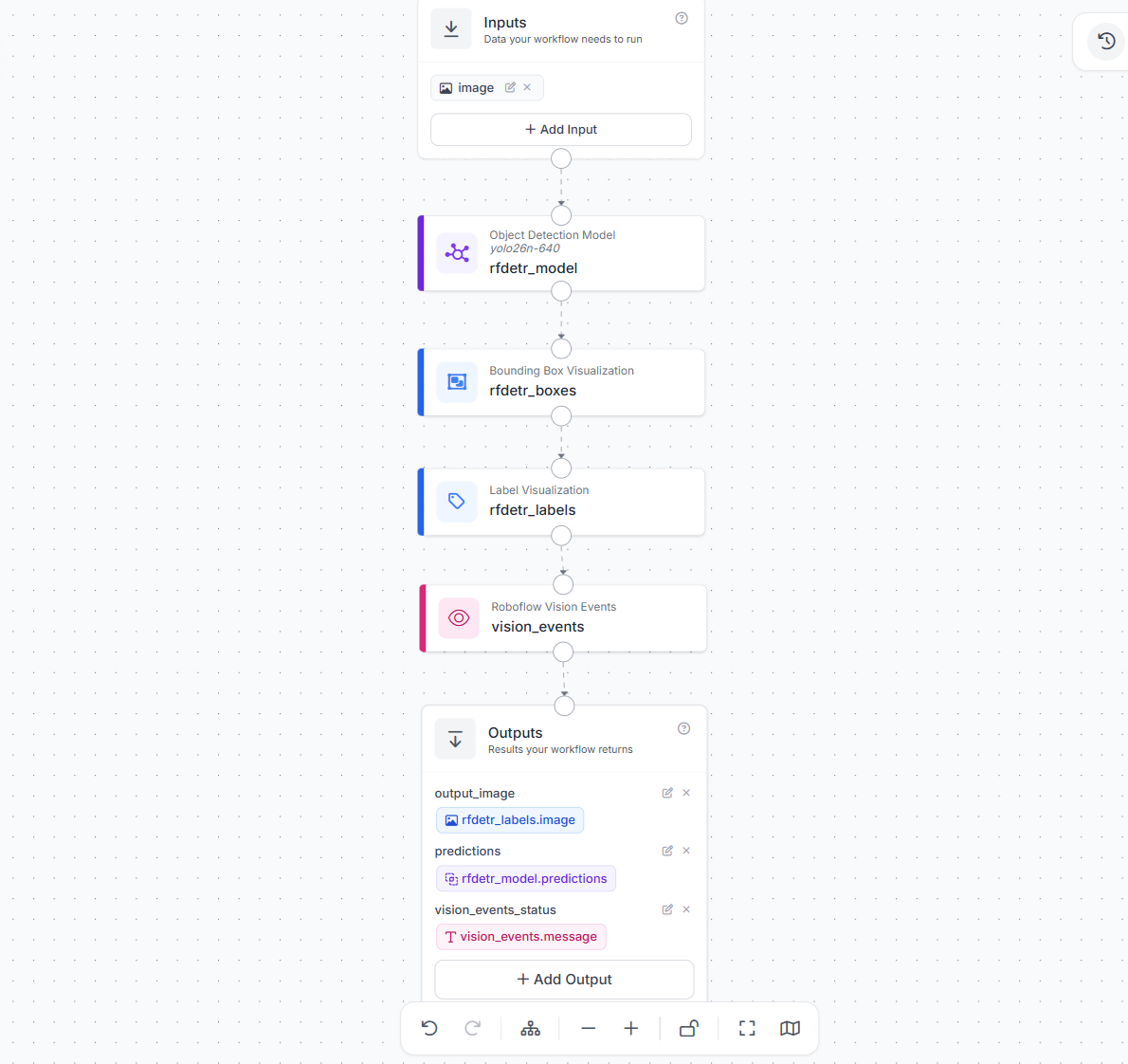
The Workflow starts with an image input. The input image is passed to the RF-DETR object detection model block, named rfdetr_model. In this example, the Workflow uses the rfdetr-small model, but you can use another RF-DETR variant depending on your speed and accuracy needs.

After the RF-DETR model runs inference, it produces object detection predictions. These predictions include bounding boxes, class labels, and confidence scores for the objects detected in the image.

The predictions are then passed through visualization blocks:

• rfdetr_boxes draws bounding boxes around detected objects.
• rfdetr_labels adds class labels and confidence information to the image.

The Workflow also includes a vision_events block. This block can be used to return event-related status or messages from the Workflow, which can be helpful when integrating the Workflow into a larger application.

Finally, the Workflow returns three main outputs:

• output_image: the image with RF-DETR bounding boxes and labels drawn on it.
• predictions: the raw RF-DETR detection results from the model block.
• vision_events_status: the message returned by the vision events block.

This Workflow gives a simple way to run RF-DETR on custom input images, visualize the detections, and inspect the raw prediction results. It can also be extended later by adding filters, custom logic, comparison blocks, or deployment-specific actions.

Step 2: Inspecting RF-DETR Model Block Execution Time with Roboflow Inference Profiling

Roboflow Workflows can be profiled when running on a local Inference Server. Profiling generates a JSON trace file that contains timing events for each Workflow step, including the RF-DETR model block used in this Workflow.

This is useful when you want to inspect how long the rfdetr_model block (or any other model block) took during a local Workflow run. However, this timing should be understood as model block execution time, not pure isolated model latency. The model block execution time may include input preparation, model inference, post-processing inside the block, output handling, and Workflow-related overhead. Here's how to do it.

Enable Workflow profiling in the local server

Create a .env file with following entry in the same directory where you start your local Inference Server:

MODEL_CACHE_DIR=/tmp/cache
ENABLE_WORKFLOWS_PROFILING=True
WORKFLOWS_PROFILER_BUFFER_SIZE=64

Then start or restart the local server with that environment file:

inference server stop
inference server start --port 9001 -e .env

The key setting is:

ENABLE_WORKFLOWS_PROFILING=True

This enables Workflow profiling inside the local Inference Server. The request must also pass enable_profiling=True; otherwise, the profiler trace will not be generated for that Workflow run. By default, profiling trace files are saved in:

./inference_profiling/

You can optionally check that profiling is enabled inside the running container:

docker ps
docker exec <CONTAINER_ID> printenv ENABLE_WORKFLOWS_PROFILING

The expected output is:

True

Run the RF-DETR Workflow with profiling enabled

Use the InferenceHTTPClient to run the Workflow against your local server:

from inference_sdk import InferenceHTTPClient

client = InferenceHTTPClient(
    api_url="http://localhost:9001",
    api_key="YOUR_ROBOFLOW_API_KEY"
)

result = client.run_workflow(
    workspace_name="YOUR_WORKSPACE_NAME",
    workflow_id="YOUR_WORKFLOW_ID",
    images={
        "image": "car.png"
    },
    enable_profiling=True,
    use_cache=False
)

print(result)

The important parts are:

api_url="http://localhost:9001"

This sends the request to your local Inference Server. Workflow profiling is intended for a self-hosted local Inference Server, not the Serverless API.

enable_profiling=True

This asks the server to generate profiling events for this Workflow run.

use_cache=False

This forces the server to fetch the latest Workflow definition instead of using a cached copy. This is helpful when you are actively editing the Workflow. If the Workflow is not changing, using the cache can be faster. Run:

python run_workflow.py

Read the profiler JSON file

After the Workflow runs, a profiler JSON file is written into:

inference_profiling/

The following script reads the newest JSON trace file and prints timing information for the RF-DETR model block:

import json
from pathlib import Path

trace_path = sorted(
    Path("inference_profiling").glob("*.json"),
    key=lambda p: p.stat().st_mtime
)[-1]

with open(trace_path, "r") as f:
    raw = json.load(f)

events = raw.get("traceEvents", raw) if isinstance(raw, dict) else raw

target_step = "rfdetr_model"

print(f"Reading trace: {trace_path}\n")

print(f"{'Step':15s} | {'Event':20s} | {'Time':>10s}")
print("-" * 52)

for event in events:
    name = event.get("name", "")
    args = event.get("args", {}) or {}
    dur_us = event.get("dur")

    if dur_us is None:
        continue

    step_text = " ".join(str(v) for v in args.values())

    if target_step in step_text and name in {"step_code_execution", "step_execution"}:
        print(
            f"{target_step:15s} | "
            f"{name:20s} | "
            f"{dur_us / 1000:8.2f} ms"
        )

Run:

python trace_rfdetr.py

What the trace output means?

The script prints output in this format:

Reading trace: inference_profiling/workflow_execution_trace_....

Step            | Event                |       Time
----------------------------------------------------
rfdetr_model    | step_code_execution  |    XX.XX ms
rfdetr_model    | step_execution       |    XX.XX ms

Each row is read from the profiler JSON file. The script does not estimate these numbers. It reads the dur field from the JSON trace event, which is stored in microseconds, then divides it by 1000 to print milliseconds. For example:

dur_us = event.get("dur")
dur_us / 1000

This converts the profiler duration from microseconds to milliseconds. If the profiler event has:

{
  "name": "step_code_execution",
  "args": {
    "step": "$steps.rfdetr_model",
    "data_size": 1
  },
  "dur": 33500
}

then the RF-DETR model block execution time is:

33500 microseconds = 33.50 ms

Understanding the profiler JSON structure

The profiler JSON file is a list of timing events. Each event describes one operation that happened during the Workflow run. A typical event looks like this:

{
  "name": "step_code_execution",
  "ph": "X",
  "pid": 1,
  "tid": 154,
  "ts": 368235240,
  "cat": "workflow_block_operation",
  "args": {
    "step": "$steps.rfdetr_model",
    "data_size": 1
  },
  "dur": 33500
}

Here is what the main fields mean,

• name , this is the operation being timed. Examples include:

workflow_definition_fetching
workflow_compilation
workflow_input_assembly
step_input_assembly
step_code_execution
step_output_registration
step_execution
outputs_construction
workflow_execution

For RF-DETR model timing, the most important events are step_code_execution and step_execution.

• ph is the Chrome trace event type. Common values are X = complete event with duration, B = begin event, E = end event. Events with "ph": "X" usually contain a dur field.
• pid is the process ID inside the container. It is mostly useful for trace visualization and is usually not needed for manual timing analysis.
• tid is the thread ID inside the container. Different Workflow steps may run on different threads.
• ts is the timestamp in microseconds. It helps place the event on the profiler timeline.
• cat is the category of the operation. Common categories include: inference_package_operation, execution_engine_operation, workflow_block_operation. workflow_block_operation is the most relevant category when inspecting model block execution.
• dur is the duration of the event in microseconds. For example, "dur": 33500 means 33.50 ms.
• args contains extra metadata about the event. Example:

"args": {
  "step": "$steps.rfdetr_model",
  "data_size": 1
}

Here $steps.rfdetr_model means the RF-DETR model block and data_size: 1 means the block processed one image or frame in that Workflow run.

Note on latency variation

The timing values in the profiler trace can vary slightly from run to run. It is normal to see the RF-DETR block take a little more or a little less time across different executions, even when using the same image. This can happen because of:

• Model warmup on the first run
• Docker or container overhead
• CPU or GPU load from other processes
• Disk or cache access
• Image size and preprocessing cost
• Python and Workflow engine scheduling
• Whether model weights were already loaded in memory

For the most reliable timing value, run the Workflow several times and average the step_code_execution value after the first warmup run. The first run is often slower because the model may need to load weights and initialize runtime resources.

What this trace does and does not tell you?

This trace tells you how long the RF-DETR model block and other Workflow steps took during the local Workflow run. It is a timing profile that helps identify where time is spent inside the Workflow. It does not measure model accuracy, precision, recall, or mAP. To measure accuracy, you need ground-truth annotations and an evaluation process. The profiler JSON contains execution timing information, not correctness information. It also should not be treated as a universal benchmark for every deployment environment. The timing depends on your local machine, hardware acceleration, RF-DETR model size, image size, server setup, cache state, and the rest of the Workflow.

Fastest Object Detection Models Conclusion

Fast object detection is not only about choosing the model with the lowest latency. The best model should provide a strong balance of speed, accuracy, and deployment performance on your own data. RF-DETR is a strong first choice in 2026, while YOLO26, YOLOv12, YOLO11, RT-DETR, RTMDet, and Roboflow 3.0 are also useful models to compare.

Using Roboflow Workflows, you can create separate Workflows for different models, run them on the same input images, and inspect their predictions. With local Roboflow Inference and Workflow profiling, you can also compare each model’s block execution time on your own device. This gives you a practical way to test multiple models trained on custom data and choose the fastest model that still gives reliable results for your specific use case, hardware, image size, and deployment pipeline.

Cite this Post

Use the following entry to cite this post in your research:

Timothy M. (Jul 1, 2026). Fastest Object Detection Models in 2026. Roboflow Blog: https://blog.roboflow.com/fastest-object-detection-models/